Countif in an Array in Google Sheets Using Vlookup and Query Combo

You can use Countif in an array in Google Sheets to return an expanded result. But it will repeat the count in each row. The best and clean looking alternative solution is using a simple Query formula.

Here in this tutorial, I am going to provide you with different Countif alternative solutions. This can also help you to understand how to combine/nest different functions.

Different Methods for Getting Countif Array Results

Query (Formula # 2 below): It provides a Countif array result that is clean looking. You will get the unique values of the selected column and its count as the second column in a new range.
The Query output mentioned in point # 1 can be achieved by using a Unique + ArrayFormula + Countif combination (Formula # 5 below).
Using the Countif function with the ArrayFormula to get an expanding result (Formula # 4 below). This solution returns the count of the selected column values against each row. For example, if the value “apple” repeats in rows 5, 7, and 8 the formula will put the count 3 in rows 5, 7, and 8.
The formula in the above point # 3 can be replaced by an Array Formula, Vlookup, and Query combination (Formula # 3 below).

Lots of messy stuff, right? But keep cool as it’s so simple with examples. I have arranged the formulas in a particular order below. I hope you will find that easy to follow.

The below examples will explain the problem with a normal Countif in an array, how a Query handles Countif, and why my combo formula is required.

How to Use Countif in an Array in Google Sheets

I have a list that shows the name of the Wimbledon Men’s Singles Champions from 2000 to 2017.

With the help of a COUNTIF formula as in cell F2, I can find the number of titles won by the player in E2.

Formula # 1:

=countif(C2:C19,E2)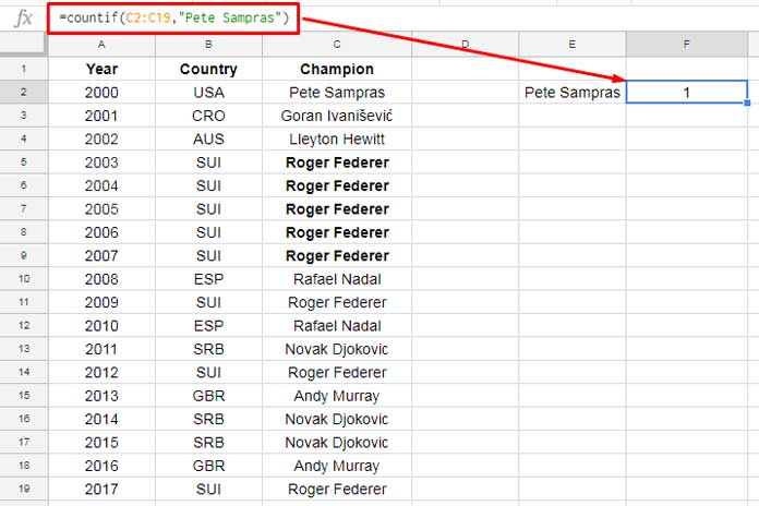

Normal countif formula without array expansion

Then how to find the number of titles won by each gentleman in Column C? Can I use Countif that way?

Of course, you can. That solution you can find under Formula # 4. But the easiest and most clean-looking solution is using a Query.

You can use a Query formula as below as an alternative to Countif in an Array in Google Sheets.

The Query for Clean Looking Countif Array Result

In cell E2 you can see my Query formula.

Formula # 2:

=query(C2:C19,"select C, count(C) group by C label count(C)''")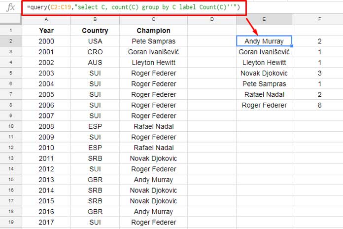

Example to Query as an alternative to Countif in Google Sheets

You can get the same above count array result by using a Unique + ArrayFormula + Countif combo. I’ll come to that later under Formula # 5.

Vlookup a Query Result to Get Countif Array Result in Google Sheets

Now we are going to use a Vlookup and Query combo. What I want to achieve is something like below.

I want the number of titles won by each player against their name itself. We can use the above Query in Vlookup to get the count in each row.

Formula # 3:

=ArrayFormula(vlookup(C2:C19,query(C2:C19,"select C, count(C) group by C label Count(C)''"),2,FALSE))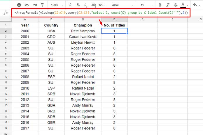

how to use Countif function in an Array in Google Sheets

Formula Explanation:

In this, I’ve used the same Query formula which you can find under Formula # 2.

Now to make you clear about the rest of the formula part, please have a look at the Vlookup syntax below.

VLOOKUP(SEARCH_KEY, RANGE, INDEX, [IS_SORTED])

Here the argument “range” is the above Query Formula # 2 which returns the name of the winners (first column) and their number of titles (second column).

The search key in Vlookup is in C2:C19. The Vlookup will search for these keys in the first column (name of the winners) in the Query result. Then the Vlookup will return the count/number of titles available in the second column of the Query result.

This combination is a must to learn as you can replace count with other aggregation functions in Query and use in Vlookup for different types of array results.

Countif Multiple Criteria Output Using the Range Twice as Range and Criteria

Formula # 4:

You can replicate the Formula # 3 result using Countif itself! Apply this formula in Cell D2 to get the same above Query and Vlookup output. It’s so simple.

=ArrayFormula(countif(C2:C19,C2:C19))

I know this formula is far better than Formula # 3. Then why this formula comes later in the order? Because I want to show you how can we use the Formula # 2 result (Query) in Vlookup as a range.

Secondly, and to your surprise, we can use this Formula # 4 to return the same result produced by Query Formula # 2!

For that, you only need to wrap the above formula with the UNIQUE function.

Formula # 5:

=ArrayFormula(unique({C2:C19,countif(C2:C19,C2:C19)}))

Conclusion

I have provided you with five formulas and all are entirely different types to help you to get Countif in an Array in Google Sheets.

If you find it difficult to understand, apply all the above steps in your own Google Sheets. If any part of this tutorial seems tough for you, please don’t hesitate to contact me via the comment form below. Enjoy!

44 COMMENTS

Radmila April 14, 2022 At 8:46 pm

Hi, I have 6000 products, with values 1-100, some are current assortment products, and some are previous assortment values.

I’m trying to count how many current and previous products have each value from 1 to 100.

I’m trying to use the countifs formula with two conditions – “ex” or “current” and value (ranging 1-100).

However, it is not working in google sheets:

=COUNTIFS('db prod'!$D:$D,E$4,'db prod'!$F:$F,$D5)

Wherein;

1. Column F on the ‘db prod’ sheet I have values 1-100, in cell D5 is value 100.
2. Column D on the ‘db prod’ sheet contains “ex,” “current” or “potential,” and E$4 contains the value “ex.”

May you help me?

- Prashanth April 17, 2022 At 2:37 pm
  
  Hi, Radmila,
  
  You can try this COUNTIFS formula.
  
  =ArrayFormula(sum(COUNTIFS('db prod'!$D:$D,{"current","ex"},'db prod'!$F:$F,$D5)))
  
Abram August 23, 2021 At 4:33 am

Hi,

I’m looking for a formula that counts a range of rows as one count if one or more cells in the range contain a specific text.

Please find my sheet for more explanation and the desired result at the bottom of this comment.

I would be very glad if you could help me.

— sample sheet link removed by admin —

- Prashanth August 23, 2021 At 11:49 am
  
  Hi, Abram,
  
  I have inserted a ‘complex’ Countif formula in cell A13.
  I hope that helps.
  N.B.: I may try to explain the formula in my coming tutorial.
  
  - Abram August 23, 2021 At 1:35 pm
    
    Thank you so much. It’s truly is a day saver.
    
    - Prashanth August 26, 2021 At 2:27 pm
      
      Hi, Abram,
      
      You can read a similar tutorial here – Find the Longest String in Each Row in Google Sheets.
      
Christophe344787 August 3, 2021 At 3:16 pm

Hi,
I am looking to reverse the count with an arrayformula of row occurrences on two columns. Could you help me?

- Prashanth August 3, 2021 At 7:19 pm
  
  Hi, Christophe344787,
  
  You may replace row(A2:A) with sort(row(A2:A),1,0).
  (twice in the formula)
  
- Prashanth August 7, 2021 At 6:33 pm
  
  Hi, Christophe344787,
  
  Here is the relevant tutorial – Reverse Running Count Simplified in Google Sheets.
  
Kermit Goodman February 19, 2021 At 12:25 am

I am looking for a way to use ARRAYFORMULA(COUNTIF(... to count occurrences of a particular value across several columns of each ROW — as opposed to counting reoccurring values all in the same column — facing the same problem, that ARRAYFORMULA(COUNTIF(A1:D99,"value") returns a single number, rather than an array showing the COUNTIF for each row. Any suggestions on how to do this?

- Prashanth February 20, 2021 At 2:37 pm
  
  Hi, Kermit Goodman,
  
  It’s possible and I do have the formula. I’ll post it soon.
  
  In the meantime, you may please consider sharing your sheet (sample) via the ‘reply’ below.
  
- Prashanth February 22, 2021 At 6:15 pm
  
  Hi, Kermit Goodman,
  
  As promised, here is the formula (tutorial).
  
  Countif Across Columns Row by Row – Array Formula in Google Sheets.
  
  In the formula, you may replace the IF part if(A2:E>=10,A2:E,) with your condition.
  
SPH November 24, 2020 At 1:44 pm

In column B, I have Stock names of about 4000 rows.

For each company, every day, I add a data point. So, a column gets added each day.

In column C, I want the last 20 days’ values separated with the comma.

As the last column keeps changing, I use the indirect function. So, the two indirect functions keep track of the shifting columns – the start point and the last point. I hope I make sense.

- Prashanth November 26, 2020 At 11:10 am
  
  Hi, SPH,
  
  We can do that using either of the below two formulas.
  
  Formula 1:
  
  =join(",",array_constrain(SORT(filter({C2:C,row(C2:C)},B2:B<>""),2,0),20,1))
  
  Formula 2:
  
  =textjoin(",",1,query(C2:C,"Select * offset "&counta(C2:C)-20))
  
  Even though the results are the same, the formulas return the result in different orders.
  
SPH November 21, 2020 At 3:50 pm

Thank you.

Another example of arrayformula challenge:

=TEXTJOIN(char(44),,indirect($A$1&row()):indirect($B$1&row()))

How to make this expand vertically?

Thanks

- Prashanth November 23, 2020 At 10:39 am
  
  Hi, SPH,
  
  I don’t understand the use of Indirect in your formula. If you explain what you are trying to do, I may be able to help you.
  
SPH November 14, 2020 At 7:24 pm

Hi,

Formula is =IF(A4="","",COUNTA(SPLIT(A4," ")))

How to make it expand vertically using arrayformula?

Thanks

- Prashanth November 16, 2020 At 2:18 pm
  
  Hi, SPH,
  
  I’ve written a new tutorial that would probably answer your query.
  
  Split and Count Words in Google Sheets (Array Formula)
  
rachel lewis September 29, 2020 At 5:06 am

I am collecting student attendance form responses for multiple groups and multiple subjects.

I want to make a checkbox if that student is signed in for that day for that subject. I am trying to use countifs but keep getting errors.

If you can help that would be amazing.

- Prashanth September 29, 2020 At 10:13 am
  
  Hi, rachel lewis,
  
  Leave a demo sheet link as an answer to this reply. I’ll try my best.
  
Jahnavi June 15, 2020 At 6:20 pm

Hi,

I want a formula for the latest occurrence for the following example

time stamp|name|choc name
10/10/2020 10:10:10|nani|dairymilk
5/4/2020 06:30:00|teja|Cadbury
10/10/2020 11:10:10|nani|kitkat
10/10/2020 12:30:10|nani|5 star
5/4/2020 06:31:00|teja|perk

This is the data in one sheet.

And in another sheet I have names and I want the latest preference of chocolate by matching the name (if I matched with “teja” I have to get “perk” if I match with “nani” I have to get “5 star”.

- Jahnavi June 15, 2020 At 6:20 pm
  
  I want it with array formula to apply to the whole range
  
  - Prashanth June 16, 2020 At 10:35 am
    
    Hi, Jahnavi,
    
    Thanks for giving me the required details.
    
    Assume the data that you have provided is in A1:C in “Sheet1”.
    
    The criteria are in A1:A in “Sheet2”
    
    Then the below Vlookup in cell B1 in “Sheet2” will take care of your requirement.
    
    =ArrayFormula(IFNA(vlookup(A1:A,sort(Sheet1!B2:C,Sheet1!A2:A,0),2,0)))
    
    If you face any issue, make a sample sheet as per the above details and share it with me.
    
Julia November 19, 2019 At 5:06 pm

I like your Arrayformula Query solution, but I can’t think of how to make it work horizontally.

So I have a Countif every time A is mentioned in a row like so:

COUNTIF A B D A F G
COUNTIF B A D F A G
COUNTIF G B D A F G
COUNTIF A A D A F A

2
2
1
4

And I would like to slap an arrayformula in front, but it’s only supposed to sum up results when it finds an A in that row, rather than all the rows. And I want any new data o to have that formula in that cell as well.

Let me know if you know how to do this, much appreciated 🙂 I’ll also keep looking for solutions.

- Prashanth November 19, 2019 At 5:39 pm
  
  Hi Julia,
  
  The range used in the test: B2:G.
  
  The formula in cell A2.
  
  =ArrayFormula(if(len(B2:B),(mmult(if(B2:G="A",1,0),transpose(column(B2:G))^0)),))
  
  Note: Assume the above data is in B2:G5. My formula expands based on values in column B. So make sure that there is no cell blank in the range B2:B5. If you want to make a cell blank, at least leave a space (tap space bar) (applicable to only in the first column, i.e. column B).
  
  This article will give you some insight into MMULT in infinite rows.
  
  Proper Use of MMULT in Infinite Rows in Google Sheets
  
  - Dale May 3, 2021 At 12:49 pm
    
    Hey Prashanth,
    
    Is there a way to get this exact formula to work with partial text lookups?
    
    - Prashanth May 7, 2021 At 11:23 am
      
      Hi, Dale,
      
      To try, please share a sheet that contains some sample data within one tab and your expected result within another tab.
      
      You can leave the URL in the reply. I won’t publish it.
      
Gonza November 6, 2019 At 9:43 pm

Hi, Prashanth

I’m looking for a function that gives a horizontal vector with an automatic variable length. let me explain myself.

I have a column A where days are put together with hours in the following order DD/MM/YYYY hh:mm:ss, but they aren’t sequential or series based on a pattern. This is updated by GPS s installed in trucks.

So whenever an event happens (no matter the frequency) it will write in column A (DD/MM/YYYY hh:mm:ss), in column B type of event, like, Engine Stop, Change of direction N S W E, Engine Start, etc, etc. Then in column C, I have the exact location of the event.

As written above, no series involved in the process, and I want a formula to count how many unique days are in column A to put that number inside a formula like the following:

=ARRAYFORMULA(SEQUENCE(1,"I need the formula to count unique days",A2,1))

- Prashanth November 7, 2019 At 11:24 am
  
  Hi, Gonza,
  
  I could understand you want to dynamically use the [columns] in SEQUENCE.
  
  Syntax:
  
  SEQUENCE(rows, [columns], [start], [step])
  
  To get the number of unique days ( to use as [columns]) from a timestamp column (here column A), you can use this formula.
  
  =ArrayFormula(count(unique(int(A2:A))))
  
  Then your above-requested formula will be as follows.
  
  =sequence(1,ArrayFormula(count(unique(int(A2:A67)))),A2,1)
  
  Note: Format the populated date (date values) to Date using Format > Number > Date.
  
  But I think you may want something like this (Max Date – Min Date) as [columns]
  
  Try both.
  
  Best,
  
Zack October 23, 2019 At 2:03 pm

Hi Prashanth,

Is it possible that I want to count occurrences of items using arrayformula with Countif function?

Example:

Item | Occurrences
apple | 3
apple | 2
apple | 1
orange | 2
orange | 1
cherry | 1

I am using this formula countif(A2:A,A2)

So, I was thinking if we can use ArrayFormula to count occurrences without specifying values such as “apple”
Thank you, 🙂

- Prashanth October 24, 2019 At 9:43 am
  
  Hi, Zack,
  
  The count of “apple” is 3, “orange” is 2 and “cherry” is 1.
  
  =ArrayFormula(if(len(A2:A),countif(A2:A,A2:A),))
  
  This Array Countif formula would return the result accordingly.
  
  Are you looking for the same output that you have specified in your comment?
  
  Please clarify.
  
  Best,
  
  - Zack October 24, 2019 At 1:09 pm
    
    Hi Prashanth,
    
    Actually “Occurrences” column is being calculated by this formula =countif(A2:A,A2)
    
    So, I was wondering if I can use an arrayformula instead of dragging the formula when a new item is added to the list?
    
    - Prashanth October 24, 2019 At 2:26 pm
      
      Hi, Zack,
      
      There is no (specific function) based arrayformula to do that. Here is a combo.
      
      This formula is for the range A2:A. You can use this formula in cell B2. It will expand down.
      
      Note: Due to some technical issues, I am unable to post the formula. I hope the image will help.
      
      Best,
      
    - Prashanth November 19, 2019 At 5:25 pm
      
      https://infoinspired.com/google-docs/spreadsheet/count-of-occurrences-in-each-row-in-google-sheets/
      
Daniel October 7, 2019 At 8:26 am

BTW, the lookup would take the same match criteria (A2) as the first criteria pair.

- Prashanth October 7, 2019 At 9:59 am
  
  Hi, Daniel,
  
  I’m in the dark 🙁
  
  Can you please share a mockup spreadsheet?
  
  Best,
  
Daniel October 7, 2019 At 8:25 am

OK, I’ve moved forward on my own, but now I have a new question. I am pulling counts with criteria, but I want to replace the day counts (7 and 10 below) with results from a Vlookup. Can it be done?

=IF(ISBLANK(A2),"",COUNTIFS(Latest!$E$2:$E,A2,Latest!$F$2:$F,""&today()-10))

Daniel October 6, 2019 At 11:20 am

Wow, I have a lot to learn. Maybe you can help. I have a sheet with tabs that represent the stages a customer moves through in our funnel, from NEW to PAID to COMPLETED the training (there are actually 7 stages, but 3 will do for example)

Their email address is the key, and it appears on each of the TABS if they have completed that stage, along with the date of completion.

For each tab, I want to basically do this type of count:

COUNT IF the email is not in any of the sheets to the right (later stages not yet reached)

Also, for an aging report, I want to add “AND DATE IS > X DAYS AGO”

Not sure how to use/combine query w/ Vlookup. Thanks for any guidance!

Mallik K September 10, 2019 At 3:51 pm

Hello Prashanth,

I need your help with the the below query.

For your above example. Let us consider three more additional columns, “Prize Money Won” that is unique value for each year and then a column, that is “Donated to Non-Profit” that is donated from the player to non – profit and then the third one would be the balance prize money that is residual of (Prize money won – Donated Amount).

The result should include the balance = total prize money – total amount donated (all titles included – group by each player).

thank you

- Prashanth September 10, 2019 At 8:45 pm
  
  Hi, Mallik,
  
  Need an example Sheet to look into the problem.
  
  Best,
  
Boudewijn July 4, 2019 At 3:01 pm

Hi there!

I have a calculation that contains a Countifs formula, and because it contains a check to see whether a date takes place in a month and year, an Arrayformula needed to be added.

I’m hoping to find a way where I don’t have to copy + paste the formula for new values.

This article almost seems to offer the solution, but I can’t really find it out… Do you know what I need to do?

This is how it looks now:

=ARRAYFORMULA(COUNTIFS(Blad1!$A:$A;$B5;year(Blad1!$E:$E);F$1;MONTH(Blad1!$E:$E);F$2))

B5 = User ID
F1 = a cell with value ‘2019’
F2 = a cell with value ‘1’ for January

- Prashanth July 5, 2019 At 10:08 am
  
  Hi, Boudewijn,
  
  You didn’t mention the cell containing your formula. Also when you copy paste the formula what changes you are expecting in the cell references in the formula.
  
  Best,
  
Rahul sinha June 3, 2019 At 1:49 pm

I want to apply a Countif formula for each row, to count the occurrences of a value every time. For this, I dragged the formula to the last row and it worked fine. But the problem arises when a new row is added automatically in the Google Sheet (due to Google Form response). The Countif formula is not added to the new row.

For this, I applied ARRAYFORMULA with Countif to automatically update the formula with the addition of the new row. It is working but the ARRAYFORMULA is giving the highest occurrence number for every match.

Please help me to solve this.

- Prashanth June 3, 2019 At 4:59 pm
  
  Hi, Rahul,
  
  I will definitely try to help you. But I want to see your source data. I know it involves privacy. So, you can make mockup data and share.