


In this tutorial, we can learn how to Vlookup part of a sentence in a list of words in Google Sheets.
How does it differ from the regular VLOOKUP formula, then?
I’ve used “Sentence” symbolically in the title. It means the length of the search key may be larger than the values in the search column.
So the regular Vlookup won’t work here.
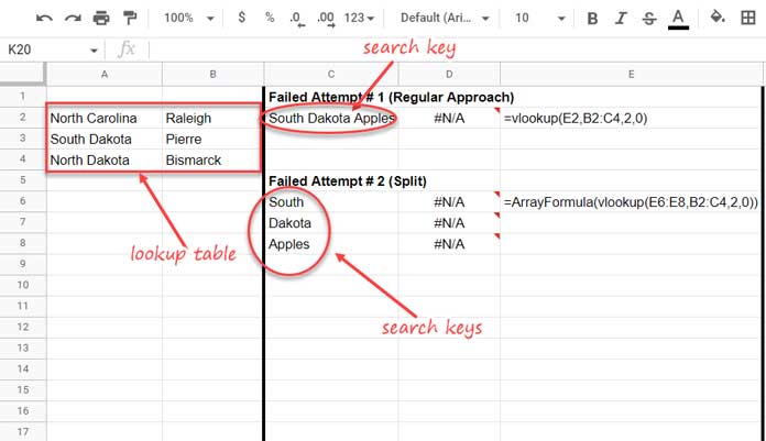
For example, “South Dakota Apples” is the search key to use in the Vlookup.
We want to search for this in a column containing a list of places; North Carolina, South Dakota, and North Dakota; and get the capital city from the next column.
If you split the sentence (search key) and use the outputs as the search keys, it won’t return the correct result. So we have to follow an entirely different approach.
That is what we are going to learn in this tutorial.
Actually, to Vlookup a sentence in a list of words, we won’t use the Vlookup function as it won’t support this.
There is a workaround that will even handle multiple search keys (sentences) in one go!
Workaround Using Countif, Filter, Len, Sort, Index, and Ifna
We can use two types of formulas to Vlookup a sentence in a list of words in Google Sheets.
One is a non-array formula that can handle one search key.
If you have multiple search keys, you must copy-paste this formula down.
The other is an array formula that takes multiple search keys and spills down its own.
Both formulas use Countif, Filter, Len, Sort, Index, and Ifna combination.
Additionally, the array formula uses a Lambda helper function to spill the result.
Drag-Down Formula to Vlookup a Sentence in a List of Words
All the functions in the combination have their role to play.
Here is the non-array formula to Vlookup (vertical lookup) a sentence in a word. Insert it in D2 and copy-paste it down as far as you want.
=ifna(index(sort(filter(B2:B,countif(C2,"*"&A2:A&"*")),filter(Len(A2:A),countif(C2,"*"&A2:A&"*")),0),1))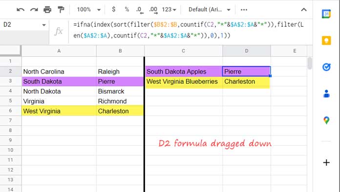
Anatomy of the Formula
The logic of this formula starts from the COUNTIF and the syntax of which is as follows.
COUNTIF(range, criterion)If you count A2:A (Countif criterion) with wildcards in cell C2 (Countif range), you will get the # 1 against all partial matching values against A2:A.
To test, use =ArrayFormula(countif(C2,"*"&$A$2:$A&"*")) in cell F2 (we require ArrayFormula when testing it independently).
The FILTER filters B2:B that matches Countif result = 1.
=filter($B$2:$B,countif(C2,"*"&$A$2:$A&"*"))I’ve removed the ArrayFormula with Countif as it’s within another array formula, i.e., Filter.
It seems enough to Vlookup a sentence in a word in Google Sheets at a glance. But it’s not so!
When using the C2 value, it’s OK. But if you use the C3 criterion, i.e., “West Virginia Blueberries,” the Countif matches Virginia and West Virginia.
So the Filter will output two capital cities, Richmond and Charleston.
The best match of the search key “West Virginia Blueberries” is “West Virginia,” not “Virginia.” So we expect Charleston as the output.
| Virginia | Richmond |
| West Virginia | Charleston |
The solution is to SORT the Filter output (B2:B) based on the length of the corresponding A2:A values in descending order.
So we will get the best possible match at the top of the filter output.
=sort(filter($B$2:$B,countif(C2,"*"&$A$2:$A&"*")),filter(Len($A$2:$A),countif(C2,"*"&$A$2:$A&"*")),0)The INDEX extracts the first value. The role of IFNA is to return blank if the Vlookup sentence match returns #N/A.
Spill Down Formula to Vlookup a Sentence in List of Words
The question here is; how to convert the non-array formula Vlookup a Sentence in List of Words formula to an array one?
It’s simple nowadays as we can do that using the Lambda functions. Here we will use MAP.
We want to use all the search keys in Vlookup, I mean in the workaround formula.
The corresponding range is C2:C. So we can use the formula in D2 as follows (D2:D must be empty beforehand).
=Map(C2:C,lambda(r,ifna(index(sort(filter($B$2:$B,countif(r,"*"&$A$2:$A&"*")),filter(Len($A$2:$A),countif(r,"*"&$A$2:$A&"*")),0),1))))That’s all about how to Vlookup a sentence in a list of words in Google Sheets.
I hope you find it helpful. Thanks for the stay. Enjoy!