We can utilize a Lambda function to sort data separated by line breaks within cells in either ascending or descending order in Google Sheets.

This approach employs a formula that utilizes a Lambda helper function. Consequently, the sorted result will generate a new data range.

Please be aware that Lambda (helper) functions can be resource-intensive compared to native functions. Therefore, use my formula approach if you don’t have data in 1000+ rows.

In my opinion, only use line breaks when necessary, as they may affect data manipulation.

Line Breaks within a Cell and How They Affect Sorting

Typically, we separate values by a delimiter such as a comma, pipe, etc., within a cell. Sometimes we may want values in multiple rows within a cell.

To achieve this, we can use the keyboard shortcut Alt+Enter (Windows) or Option+Enter (Mac) in Google Sheets.

For example, if you want three lines in cell A1, and they are “23 Main Street,” “Anytown,” and “IN 12345,” type “23 Main Street” and hit Alt+Enter or Option + Enter, depending on your OS. Then type “Anytown,” and apply the keyboard shortcut, and enter “IN 12345.”

By doing this, you have created two new lines within cell A1 by inserting line breaks (newline characters). The line break character that you applied using the keyboard shortcut is the one you get when you enter the formula =CHAR(10).

Related: Start New Lines Within a Cell in Google Sheets – Desktop and Mobile.

So, in formulas, you can use CHAR(10) to insert or match line breaks, and we will make use of it in sorting data separated by line breaks within Google Sheets cells.

Although line breaks enhance readability and maintain the integrity of the data within the cell, there are drawbacks when filtering, sorting, conditional formatting, and manipulating data.

In this tutorial, we will address sorting data that contains line breaks. First of all, let’s see how line breaks affect sorting.

Sample Data and Sorting Behavior with Line Breaks in Cells

In the following example, I want to sort the sample data in the range A2:B. First, sort column A2:A in ascending order, and then sort column B2:B in descending order.

There are line breaks in many cells in column B. You can see multiple lines in cells B2, B3, B4, B6, and B7. When sorting, I want them sorted within cells in descending order, and column A in ascending order.

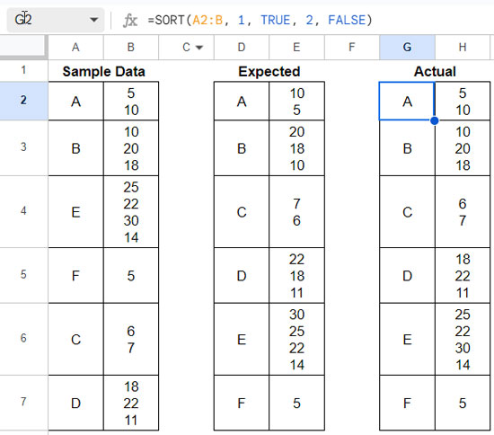
This is the formula in cell G2:

=SORT(A2:B, 1, TRUE, 2, FALSE)

It simply sorts column A in ascending order, and there is no impact on sorting data separated by line breaks in column B.

Formula Explanation

Syntax of the SORT Function:

SORT(range, sort_column, is_ascending, [sort_column2, …], [is_ascending2, …])

Where:

• range: A2:B
• sort_column: 1
• is_ascending: TRUE, which means sort column 1 in the range in ascending order.
• sort_column2: 2
• is_ascending2: FALSE, which means sort column 2 in the range in descending order.

We need to follow a different approach for sorting data when line breaks are present in one or more columns in Google Sheets. Let’s go to those formulas.

Formula to Sort Data Separated by Line Breaks in Google Sheets

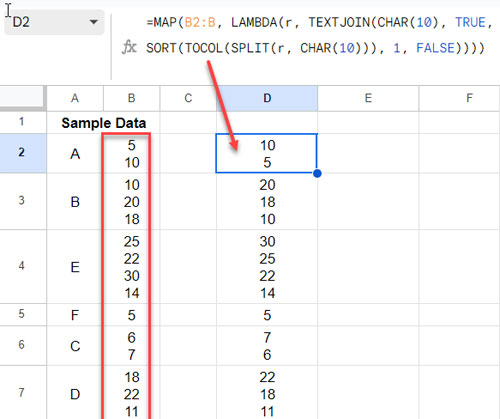
In the above example, I’ve used the following formula in cell D2 to sort data separated by line breaks in Google Sheets:

=IFERROR(SORT(
      HSTACK(
         A2:A, 
         MAP(B2:B, LAMBDA(r, 
         TEXTJOIN(CHAR(10), TRUE, SORT(TOCOL(SPLIT(r, CHAR(10))), 1, FALSE))))
      ), 1, TRUE
))

Understanding this formula is crucial for its application with data containing line breaks in a different column or multiple columns.

Formula Breakdown

The formula involves the use of several functions: IFERROR, SORT, HSTACK, MAP, TEXTJOIN, TOCOL, SPLIT, and CHAR.

MAP Part:

The key aspect of the formula is the following MAP expression:

MAP(B2:B, LAMBDA(r, TEXTJOIN(CHAR(10), TRUE, SORT(TOCOL(SPLIT(r, CHAR(10))), 1, FALSE))))

This sorts the data in column B, separated by line breaks, in descending order.

Syntax of the MAP Function:

MAP(array1, [array2, …], LAMBDA([name, …], formula_expression))

The MAP function creates a new array by applying a lambda function to each value in B2:B, where each value is represented by the identifier r.

The lambda function, LAMBDA(r, TEXTJOIN(CHAR(10), TRUE, SORT(TOCOL(SPLIT(r, CHAR(10))), 1, FALSE))), operates on each value r:

• SPLIT(r, CHAR(10)): Splits at the newline character (CHAR(10)).
• TOCOL(SPLIT(r, CHAR(10))): Transforms the result into a single column.
• SORT(TOCOL(SPLIT(r, CHAR(10))), 1, FALSE): Sorts this result in descending order.
• TEXTJOIN(CHAR(10), TRUE, …): Combines the result using the newline character.
• MAP repeats this operation for each row in the range B2:B.

HSTACK Part:

The HSTACK function appends the range A2:A with the MAP result, which is the sorted column data.

HSTACK(A2:A, MAP_expression)

Outer SORT:

The outer SORT formula then sorts column A in ascending order.

SORT(HSTACK(A2:A, MAP_expression), 1, TRUE)

Finally, IFERROR removes any error values, if present.

Advanced Tips: Sorting Data with Line Breaks in Multiple Columns

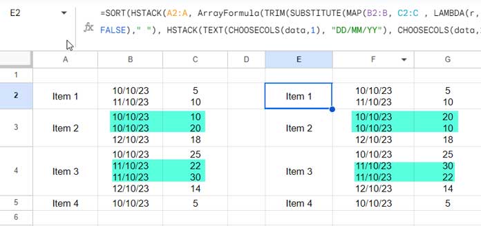
In the following example, I have item names in column 1, the date of receipt in column B, and corresponding quantities in column C.

Columns B and C contain line breaks in cells to improve the readability of the data. I mean, if an item is received multiple times, dates are entered within one cell and corresponding quantities within another cell by inserting line breaks.

As usual with line breaks, sorting is a problem here.

I want to sort items based on their receipt and quantity. If an item is received multiple times in a day, I want the maximum quantity at the top.

How do we sort data separated by line breaks within cells in multiple columns?

The Generic Formula will be:

=SORT(HSTACK(range_1_without_newlines, ranges_2_3_with_newlines), 1, TRUE)

In our example, column 2 contains dates and column 3 contains numbers. So in the generic formula, replace range_1_without_newlines with A2:A and ranges_2_3_with_newlines with the following formula:

ArrayFormula(TRIM(SUBSTITUTE(MAP(B2:B, C2:C , LAMBDA(r, rr, QUERY(LET(data, IFERROR(SORT(HSTACK(TOCOL(SPLIT(r, CHAR(10))), TOCOL(SPLIT(rr, CHAR(10)))), 1, TRUE, 2, FALSE)," "), HSTACK(TEXT(CHOOSECOLS(data, 1), "DD/MM/YY"), CHOOSECOLS(data, 2)))&CHAR(10),,9^9))), CHAR(10)&" ", CHAR(10))))

Note: If column 2 in your table is text or numbers, remove the highlighted part in the formula which essentially formats date value to date.

Formula Logic and Breakdown

I am breaking down the formula for ranges_2_3_with_newlines.

In the formula, there are two arrays in the MAP function: B2:B and C2:C. The corresponding identifiers for each row are represented by r and rr.

The TOCOL + SPLIT operation is applied to both arrays separately:

TOCOL(SPLIT(r, CHAR(10)))
TOCOL(SPLIT(rr, CHAR(10)))

The HSTACK function appends these data horizontally, and the SORT function is then used to sort column 1 (dates) in ascending order and column 2 (quantities) in descending order.

SORT(HSTACK(TOCOL(SPLIT(r, CHAR(10))), TOCOL(SPLIT(rr, CHAR(10)))), 1, TRUE, 2, FALSE)

Next, the IFERROR function is employed to replace error values in blank rows with " " characters:

IFERROR(SORT(HSTACK(TOCOL(SPLIT(r, CHAR(10))), TOCOL(SPLIT(rr, CHAR(10)))), 1, TRUE, 2, FALSE)," ")

The LET function is used to name this result as data, and each column is extracted using CHOOSECOLS. This is done to format dates in the column #1.

LET(data, IFERROR(SORT(HSTACK(TOCOL(SPLIT(r, CHAR(10))), TOCOL(SPLIT(rr, CHAR(10)))), 1, TRUE, 2, FALSE)," "), HSTACK(TEXT(CHOOSECOLS(data, 1), "DD/MM/YY"), CHOOSECOLS(data, 2)))

Line break characters are added, and the QUERY function is used to join rows.

QUERY(...&CHAR(10),,9^9)

MAP repeats this operation for each row in the range B2:C.

Finally, TRIM and SUBSTITUTE functions are applied to remove blank newlines and space characters.

Conclusion

In the above discussion, we explored two different examples of sorting data separated by line breaks within Google Sheets cells.

In the first example, we have data in two columns, with line breaks in the second column. Conversely, in the second example, there are three columns, and columns 2 and 3 contain line breaks.

In the second example, it’s designed for advanced users. Beginners might find it a bit tricky to change the formula depending on the type of data—whether it’s date, number, or text. I’ve explained things and marked where you can make adjustments.

If you have any questions or are unsure about something, feel free to ask in the comments.