We will utilize a combination formula (highlight rule) to highlight today’s date and the next n cells below in a Google Sheets calendar.

Many of you may be familiar with the process of highlighting today’s date in a sheet, whether it is part of a calendar or not in Google Sheets. This is commonly achieved using the TODAY() function.

However, in the context of a calendar, where each week is separated by rows—comprising a total of six rows with dates and an equal number of rows between each week—matching today and highlighting today plus the next n cells becomes a bit more complex.

Let’s delve into an example to illustrate the process.

Pre-Requisites

In many calendars, dates are often represented as numbers, such as 01, 02, 03, etc., rather than in a formatted date style like 01/01/2024, 02/01/2024, 03/01/2024, and so forth.

In both cases, whether using formatted dates or numerical representation, we can match today’s date and highlight the next n cells below that date.

However, if you are using a calendar template that uses numbers to represent dates, and the underlying value (visible in the formula bar when you click the cell) is also a number, the conventional date highlighting method may not be applicable.

If you’re interested, you can access my dynamic yearly calendar template by clicking the link below. If you choose to use this template, please remove any existing highlighting.

Calendar [Dynamic]

How to Highlight Today and N Cells Below in a Google Sheets Calendar

For example, I’m using the aforementioned calendar template. I hope you have already seen the preview by clicking the button above.

Here is the screenshot for those who don’t want to use that calendar.

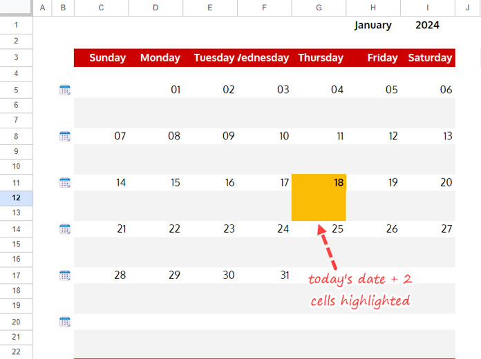
As you can see, the calendar dates are in the range C5:I20, where Week #1 is in C5:I5, Week #2 in C8:I8, Week #3 in C11:I11, Week #4 in C14:I14, Week #5 in C17:I17, and Week #6 in C20:I20. These are real dates formatted as numbers.

There will be a maximum of 5 weeks in a month, but the dates are spread across six rows because of the offset days in the first row to match the days of the week.

I’ve explained this to help you understand the area (apply to range) that we want to use in the conditional formatting. Needless to say, it’s the range C5:I20.

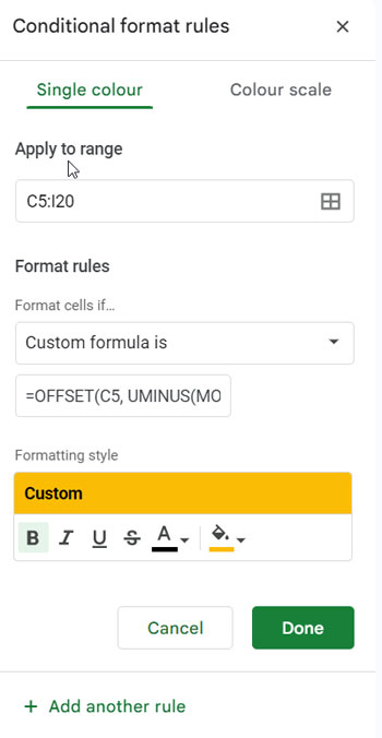
So, you need to write the formula for cell C5 and use ‘Apply to range’ C5:I20 in the conditional formatting. The formula will test each cell in the range and apply the highlighting accordingly.

For highlighting today’s date in the above Google Sheets calendar, you can use the following formula:

=C5=TODAY()

Applying the Highlight Rule:

1. Click Format > Conditional Formatting.
2. Under “Apply to range,” enter C5:I20, which is the actual calendar range.
3. Under “Format rules,” select “Custom formula is” and enter the above formula.
4. Under “Formatting style,” select your choice of highlighting.
5. Click Done.

Now, let’s proceed to highlight today’s date and the next n cells below in a Google Sheets calendar.

First and foremost, you must count the number of rows between each week. In our template, it’s two rows each.

You can use the following formula to highlight today’s date and the next 2 cells below it:

=OFFSET(C5, UMINUS(MOD(ROW(C5)-5, 3)), 0)=TODAY()

To apply, replace =C5=TODAY() with the formula provided just above within the Conditional Formatting settings.

How Can I Adjust the Formula to Suit My Calendar and N Cells?

Replace C5 with the very first cell in the calendar where Week #1 dates are present. In my calendar, it is cell C5.

Replace -5 with the row number of the very first cell of your calendar.

For example, if your calendar starts at B2, you should use the below formula:

=OFFSET(B2, UMINUS(MOD(ROW(B2)-2, 3)), 0)=TODAY()

The above formula is for highlighting today + the next 2 cells below it. To change from the next two to the next six, replace 3 with 7. So the formula will become:

=OFFSET(B2, UMINUS(MOD(ROW(B2)-2, 7)), 0)=TODAY()

Highlight Today + Next N Cells: Formula Breakdown

The formula used above to highlight today + the next n cells consists of two parts:

The first part will return the date from the non-blank cell above in all cells in the range.

=OFFSET(C5, UMINUS(MOD(ROW(C5)-5, 3)), 0)

The second part is the function that returns today’s date.

=TODAY()

The formula matches part 1 = part 2 and highlights the cells that evaluate to TRUE.

Now, let’s break down what the part #1 formula does.

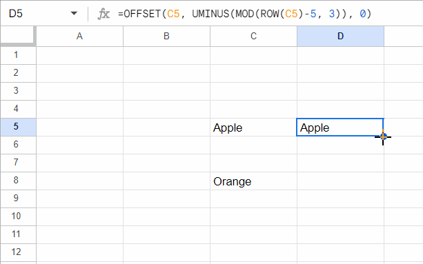
In any blank sheet, enter any two values in cells C5 and C8, for example, the text “Apple” in cell C5 and “Orange” in cell C8.

In cell D5, enter the part #1 formula and copy it down.

You can see that the formula retrieves the values in three rows: the current row and the next two rows below.

The formula adheres to the following OFFSET function syntax:

OFFSET(cell_reference, offset_rows, offset_columns, [height], [width])

Where:

• cell_reference: C5
• offset_rows: UMINUS(MOD(ROW(C5)-5, 3))
• offset_columns: 0

The key is the offset_rows which returns 0 in the current row, -1 in the second row, and -2 in the third row. When you drag it further down, it will again return the same pattern of 0, -1, and -2.

This causes the OFFSET to return the same value in three rows (current row + next two rows).

The ROW function returns the row numbers starting from 0, 1, 2, 3, 4, 5, …

We have used the MOD function to convert this to 0, 1, 2, 0, 1, 2, …

UMINUS converts it to negative numbers, with the sign reversed. The OFFSET function offsets from cell C5 accordingly.

That’s the logic behind highlighting today and the next n cells in a Google Sheets calendar.

Resources

In this tutorial, you have two formulas: one for highlighting today’s date and the other for highlighting today’s date and the next n cells below. For additional conditional formatting rules involving dates, please refer to these tutorials:

1. How to Highlight Next N Working Days in Google Sheets
2. Highlight Duplicate Values Based on Occurrence Days in Google Sheets
3. Highlight Same Day Duplicates in Google Sheets
4. How to Highlight Cells Based on Expiry Date in Google Sheets
5. Date-Related Conditional Formatting Rules in Google Sheets
6. Highlight Duplicates within the Same Month in Google Sheets