With the help of a custom formula, we can highlight duplicates that fall within the same month in Google Sheets.

For example, in real life, this will help us quickly find all the items we have procured more than once in the same month.

For example, if we purchased Cement on 15/08/2022, 26/08/2022, and 27/08/2022, the rule will highlight the last two records since they are duplicates.

There are many built-in rules for highlighting records based on dates, e.g., “date is,” “date is before,” and “date is after.”

But no rules to highlight duplicates that fall within the same month in conditional formatting in Google Sheets.

So let’s code one. Also, please note that the rule might vary slightly depending on the number of columns in your range.

We will learn all the techniques below, and let’s start with the basic formula.

Highlight Duplicates within the Same Month – Two Columns

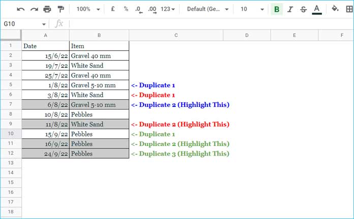
You can find a two-column dataset in the below screenshot.

I’ve used a conditional formatting formula to highlight duplicate items (column B) based on the month (column A).

Please check my notes in column C. When highlighting, the format rule excludes the first instance.

In August, we purchased Gravel 5-10 mm twice (rows # 5 and 7) and White Sand also twice (rows # 6 and 9).

In November that year, we purchased Pebbles thrice (rows # 10, 11, and 12).

So when we highlight the duplicates within the same month, the rule should highlight rows 7, 9, 11, and 12. I mean the occurrences greater than 1.

Format Rule and Applying It

Custom Format Rule (Two Columns):

=ArrayFormula(countifs($B$2:$B2,$B2,eomonth($A$2:$A2,0),eomonth($A2,0),row($B$2:$B2),"<="&row($B2)))>1

How to Apply it in Google Sheets?

You can use this rule for A2:A, B2:B, A2:B, or A2:Z. Then how to apply it in Google Sheets?

Follow the below steps to apply the custom rule to highlight duplicates within the same month in Google Sheets.

1. Select A2:B or any range mentioned above.
2. Head into Format > Conditional formatting.
3. Under Format Rules, select “Custom Formula Is” from the drop-down.
4. Copy the above code (format rule) and paste it into the blank field.
5. Use the default formatting style or customize it.
6. Select Done.

The Logic Behind Highlighting Duplicates within the Same Month

To understand the COUNTIFS formula (Yep! the above code is based on this function), please do as follows.

Copy-paste the above code in cell C2 and then edit it to remove the >1 in the last part of it.

Then drag down the fill handle (the small blue box at the bottom-right corner of cell C2) until you reach row # 12.

If the formula returns >1 in any cell, those records fall under duplicates within the same month category.

It means that to highlight the duplicate items that fall within the same month, we should highlight the rows where the formula returns >1.

The >1 in the last part of the formula acts as a logical test. It will return TRUE for >1 and FALSE for 1.

Google Sheets Conditional Formatting highlights the TRUE rows.

As a side note, remove the eomonth($A$2:$A2,0),eomonth($A2,0), parts and >1 from the formula to get the running count.

The Rule for More than Two Columns

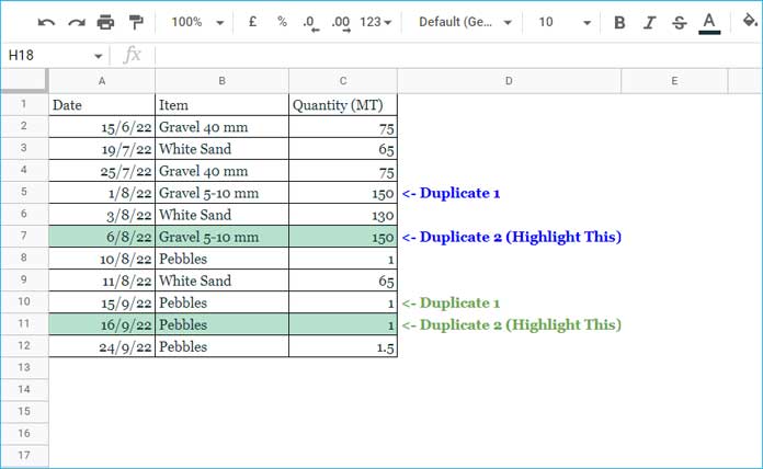
Assume we have added a quantity column and want to include that as a criterion within the format rule.

So, when highlighting duplicates within the same month, the items and their quantities also must be considered.

Please see the screenshot below.

Below, I am talking about exceptions.

As you case see, the White Sand repeats twice in August (rows # 6 and 9). But their quantities are different, so, excluded.

In the case of Pebbles, it appears thrice in November (rows # 10, 11, and 12). But the quantities are only matching in rows # 10 and 11. So the rule should highlight row # 11 only.

How to include the quantity in the code above?

Custom Format Rule: (Three Columns)

=ArrayFormula(countifs($B$2:$B2,$B2,eomonth($A$2:$A2,0),eomonth($A2,0),$C$2:$C2,$C2,row($B$2:$B2),"<="&row($B2)))>1

If you want to include additional columns, follow the above technique.

That’s all about how to highlight duplicates that fall within the same month in Google Sheets.

Thanks for the stay. Enjoy!