You can use a combination formula with WORKDAY.INTL as the key function to highlight the next N working days from a specific date in Google Sheets.
This formula requires you to specify:
- The number of business days to highlight.
- The weekends.
- Any specific holidays to exclude.
These details will be incorporated into the formula, as explained below.
How Highlighting Next N Working Days Is Useful
Sometimes, you may need to commit to clients or stakeholders that you’ll complete tasks within the next 3, 7, or 10 working days from a specific date.
In such cases, you might want to highlight rows in your dataset where the task dates fall within the next N working days. Working days exclude weekends and holidays, making this functionality especially useful for accurate scheduling.
Example: Highlighting Next N Working Days
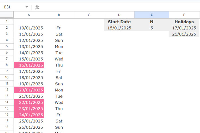
Assume the list of dates is in column A2:A.
- Enter the specific start date in D2. This could be
=TODAY()or any other date. - In E2, input the number of business days to highlight (e.g., 5).
- Use F2:F to specify holidays to exclude from the highlighting.
Now, use the following custom formula in conditional formatting:
=AND(
   ISBETWEEN(
      A2,
      WORKDAY.INTL($D$2, 1, "0000011", TOCOL($F$2:$F, 1)),
      WORKDAY.INTL($D$2, $E$2, "0000011", TOCOL($F$2:$F, 1))
   ),
   NOT(ISNUMBER(XMATCH(WEEKDAY(A2, 2), {6; 7}))),
   NOT(ISNUMBER(XMATCH(A2, TOCOL($F$2:$F, 1))))
)
This formula highlights the next 5 business days from the date in D2, excluding the holidays in F2:F. Here, “0000011” defines Saturday and Sunday as weekends.
Applying the Rule
- Select the range A2:A (the dates to be highlighted).
- Go to Format > Conditional formatting.
- Under Format rules, choose Custom formula is and paste the formula above.
- Select your preferred formatting style and click Done.
Now, the specified range will highlight the next N working days.
Customizing Weekends in the Formula
The formula uses a string to specify weekends within the WORKDAY.INTL function. The string contains seven characters where 0 represents a workday and 1 represents a weekend. For example:
"0000011": Saturday and Sunday as weekends."0000110": Friday and Saturday as weekends.
If you change the weekend string, remember to update:
- Both occurrences of WORKDAY.INTL in the formula.
- The array constants
{6; 7}for the weekend days. For example, if your weekends are Friday and Saturday, replace it with{5; 6}.
Here’s the updated formula for Friday and Saturday weekends:
=AND(
   ISBETWEEN(
      A2,
      WORKDAY.INTL($D$2, 1, "0000110", TOCOL($F$2:$F, 1)),
      WORKDAY.INTL($D$2, $E$2, "0000110", TOCOL($F$2:$F, 1))
   ),
   NOT(ISNUMBER(XMATCH(WEEKDAY(A2, 2), {5; 6}))),
   NOT(ISNUMBER(XMATCH(A2, TOCOL($F$2:$F, 1))))
)
How the Formula Works
Logical Expression 1:
ISBETWEEN(A2, next_n_start, next_n_end)WORKDAY.INTL($D$2, 1, "0000011", TOCOL($F$2:$F, 1)): Calculates the start date of the next N working days.WORKDAY.INTL($D$2, $E$2, "0000011", TOCOL($F$2:$F, 1)): Calculates the end date of the next N working days.- ISBETWEEN checks if the date in A2 falls within this range.
Logical Expression 2:
NOT(ISNUMBER(XMATCH(WEEKDAY(A2, 2), {6; 7})))Returns TRUE if the date in A2 is not a weekend.
Logical Expression 3:
NOT(ISNUMBER(XMATCH(A2, TOCOL($F$2:$F, 1))))Returns TRUE if the date in A2 is not a holiday.
If all conditions are TRUE, the formula highlights the cell.
Conclusion
Highlighting the next N working days helps you stay on top of deadlines and plan tasks more effectively by accounting for weekends and holidays. With WORKDAY.INTL and a well-structured conditional formatting rule, you can dynamically track upcoming business days based on your requirements.
For more ways to apply conditional formatting to dates, schedules, and dynamic ranges, explore the Ultimate Guide to Conditional Formatting in Google Sheets, where you’ll find a wide range of related techniques.


