When managing events, projects, or schedules, it’s often crucial to identify the earliest upcoming dates. In this tutorial, I’ll show you how to highlight the earliest event based on a date column in Google Sheets—whether you’re tracking event start dates or managing multiple bookings.
We’ll begin with a basic example where we highlight the earliest event from all entries. Then, we’ll move on to a real-world scenario where an event has multiple bookings, and I’ll show you how to highlight the earliest booking for each event individually.
Whether you’re managing conference schedules, flight bookings, or event registrations, this guide will help you organize your data and easily identify key dates with a glance.
Example 1: Highlight Earliest Events Based on Date
Sample Data (A1:B):
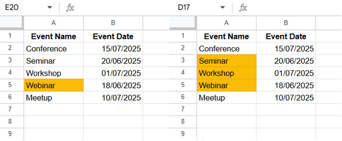
| Event Name | Event Date |
| Conference | 15/07/2025 |
| Seminar | 20/06/2025 |
| Workshop | 01/07/2025 |
| Webinar | 18/06/2025 |
| Meetup | 10/07/2025 |
In this example:
- The earliest event based on the “Event Date” is Webinar (2025-06-18).
- If you’re highlighting just the earliest event, you would highlight “Webinar.”
- If you want to highlight the top 3 earliest events, you would highlight Webinar, Seminar, and Workshop.
Steps to Highlight the Earliest Event:
- Identify the date column and the range you want to highlight. You can highlight the date column, the event column, or both.
- For this example, the date column is B, and the event column is A. We’ll highlight column A (Event Name) based on the earliest event.
- Select A2:A to highlight the event column. You can also select B2:B or A2:B depending on your needs.
- Click Format > Conditional Formatting.
- Under Format Rules, select “Custom formula is“.
- Enter the following formula to highlight the earliest event:
=AND($B2<>"", $B2=MIN($B$2:$B)) - Choose a highlight color.
- Click Done.
This formula checks whether the current row’s date is not empty and matches the minimum date in the column.
Highlighting the Top 3 Earliest Events:
If you want to highlight the earliest three events, use this formula:
=AND($B2<>"", XMATCH($B2, ArrayFormula(SMALL($B$2:$B, {1, 2, 3})))){1, 2, 3}controls the smallest three event dates.
This formula checks whether the current cell in column B is not empty and matches one of the smallest three dates.
Example 2: Highlight the Earliest Booking for Each Event
In this scenario, events may have multiple bookings, and you need to highlight the earliest booking for each event. This is particularly useful in:
- Event management: Quickly identify who booked first for VIP access, early bird perks, or seating priority.
- Hotel or venue bookings: Easily spot the first reservation to be honored.
- Ticket sales: Identify the first booking for better seating or discounts.
- Internal scheduling: Determine which department gets the meeting room first.
Sample Data:
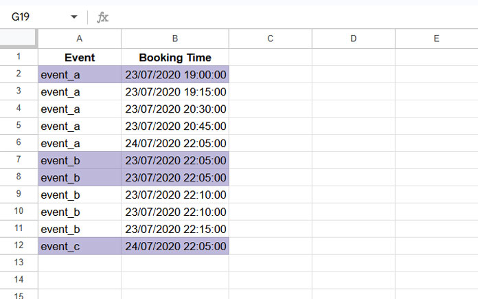
| Event | Booking Time |
| event_a | 23/07/2020 19:00:00 |
| event_a | 23/07/2020 19:15:00 |
| event_a | 23/07/2020 20:30:00 |
| event_a | 23/07/2020 20:45:00 |
| event_a | 24/07/2020 22:05:00 |
| event_b | 23/07/2020 22:05:00 |
| event_b | 23/07/2020 22:05:00 |
| event_b | 23/07/2020 22:10:00 |
| event_b | 23/07/2020 22:10:00 |
| event_b | 23/07/2020 22:15:00 |
| event_c | 24/07/2020 22:05:00 |
To highlight the earliest booking for each event, follow these steps:
- Select the event column (A2:A), the booking column (B2:B), or both.
- Click Format > Conditional Formatting.
- Under Format Rules, choose “Custom formula is“.
- Enter the following formula:
=AND($B2<>"", XMATCH(ROW($B2), FILTER(ROW($A$2:$A), $A$2:$A=$A2, $B$2:$B=MINIFS($B$2:$B, $A$2:$A, $A2))))
Formula Breakdown:
- MINIFS($B$2:$B, $A$2:$A, $A2): Finds the smallest date for the current event.
- FILTER(ROW($A$2:$A), $A$2:$A=$A2, $B$2:$B=…): Filters the row numbers where the event matches and the date is the smallest.
- XMATCH(ROW($B2), …): Matches the current row number with the filtered results.
This formula highlights the row where the current row is not empty and matches the earliest booking for each event.
Why This Method Is Useful
Using this approach, you’ll quickly identify the earliest events or earliest bookings in your Google Sheets, making it easier to prioritize tasks, allocate resources, or make decisions based on the first bookings or earliest events.
Conclusion
Highlighting the earliest events or bookings helps you quickly identify priority items, whether you’re managing schedules, reservations, or registrations. With a combination of MIN, SMALL, and MINIFS, you can apply flexible conditional formatting rules for both simple lists and grouped data.
To learn more ways to highlight dates, rankings, and dynamic conditions, visit the Ultimate Guide to Conditional Formatting in Google Sheets, where you’ll find a complete collection of related tutorials.


