Google Sheets is an online Spreadsheet solution. Still, it runs fast and offers plenty of functions and commands to manipulate data. But similar to other Spreadsheet solutions, we should know how to handle duplicates in cells for effective data manipulation. One way is using conditional formatting.

I am focussing in this tutorial on highlighting same-day duplicates in Google Sheets.

I’ll also explain how to remove the highlighted values properly in Google Sheets. You should know how to keep the first occurrences of values while removing the rest.

You may require 4 similar types of conditional format rules for highlighting same-day duplicates in Google Sheets. Let me come to that first.

Assume a customer sends two requests for one ‘same’ item in a day, or there are two or more entries of the same item in a customer’s name on a particular date.

You can flag such entries as duplicates using my first conditional format rule. It may involve a date or timestamp column, a customer name or ID column, and a product or item column.

We will use the second rule when we don’t have a customer name or ID column. What about the other two rules?

It’s just the extension of the above two rules. Use them with multiple product or item columns. You will understand them from my four examples below.

There are four highlight rules, and here are the corresponding data formats.

1. Date, ID, Value (field labels of columns).
2. Date, ID, Value1, Value2, Value3, … (field labels of columns).
3. Date, Value (field labels of columns).
4. Date, Value1, Value2, Value3, … (field labels of columns).

My last post was about filtering same-day duplicates that involve somewhat complex formulas. When it comes to conditional formatting, things are not so complex.

It’s because we are required to write the rule for the first cell in the range to test, and Sheet will do the test for the rest.

Highlight Same Day Duplicates With ID Column in Google Sheets

An easy way to identify persons who have bought/sold/requested the same item/service multiple times in a day in a dataset.

Example 1: Date, ID, and Value Columns

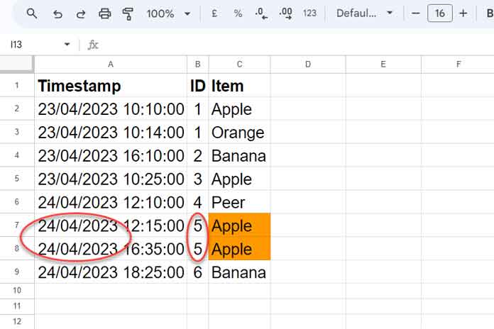
In the above example, the formula highlights the same-day duplicates, i.e., “Apple,” in column C. It repeats twice on 24/04/2023 for the same ID number.

That means ID # 5 bought “Apple” twice on the same day. You can use the same approach to highlight OPD numbers who have been given the same medicine more than once on the same day.

You can use the below formula rule.

=countif(filter($C$2:$C,int($A$2:$A)=int($A2),$B$2:$B=$B2),C2)>1

Please follow the below steps to apply this same-day conditional format rule in Google Sheets.

1. Select C2:C (the range to apply the formatting).
2. Go to the menu Format > Conditional formatting.
3. Under Format rules, select “Custom formula is.”
4. Copy-paste the above formula (rule) into the given field.
5. Click on the paint bucket under “Format style” to apply your chosen color fill.
6. Click on the “Done” button.

Example 2: Date, ID, and Multiple Value Columns

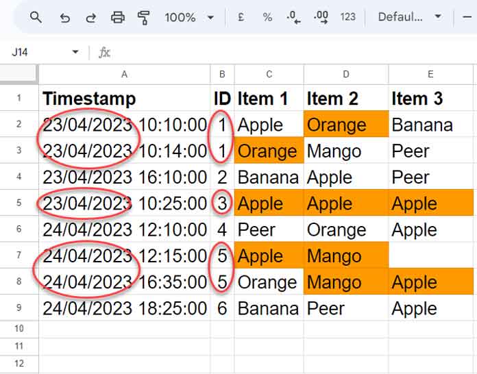
In the above example, there are four duplicates, two each on 23/04/2023 and 24/04/2023.

ID # 1 bought “Orange” twice, and ID # 3 bought “Apple” thrice. So, “Orange” and “Apple” are duplicate purchases on 23/04/2023.

On 24/04/2023, ID # 5 bought “Apple” twice and “Mango” twice. So they are duplicates.

Imagine the IDs are OPD numbers and fruit names are medicines. You will understand how useful highlighting the same-day duplicates in Google Sheets is.

To highlight as above, apply the below rule for the range C2:E as per the instructions (6 points) furnished under example # 1 above.

=countif(filter($C$2:$E,int($A$2:$A)=int($A2),$B$2:$B=$B2),C2)>1

This formula has only one difference when you compare it with example # 1. The filter range is $C$2:$C in example # 1 and $C$2:$E in example # 2.

Highlight Same Day Duplicates Without ID Column in Google Sheets

It’s an easy way to identify multiple entries of the same items in a column or row.

Example 3: Date and Value Columns

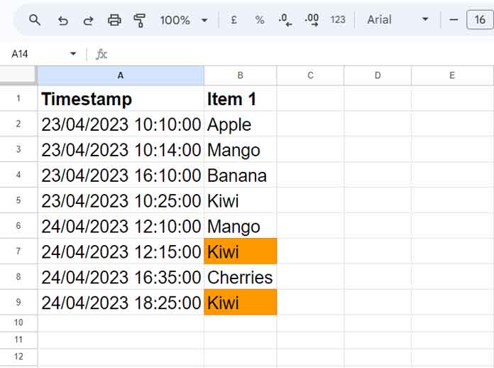
In the above example, we don’t have an ID column. We want to highlight duplicate entries having the same date or timestamp.

How do we do that?

Apply the following same-day highlight rule for the range B2:B.

=countif(filter($B$2:$B,int($A$2:$A)=int($A2)),B2)>1

Example 4: Date and Multiple Value Columns

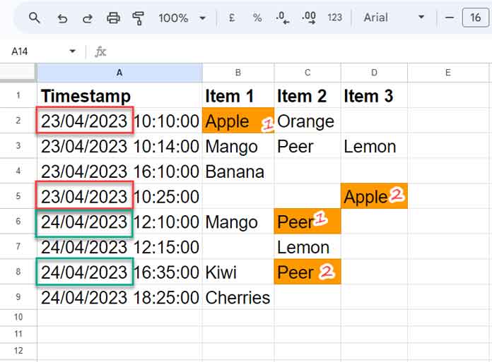
It is similar to example 3 above. The only difference is we have multiple value columns this time.

Same-day duplicates can be in one row or multiple rows. But that doesn’t make the highlight rule complex.

You are only required to modify $B$2:$B in the example # 3 rule with $B$2:$D.

=countif(filter($B$2:$D,int($A$2:$A)=int($A2)),B2)>1

Highlight Same Day Duplicates and Removing Occurrences

We have already discussed the highlighting part. How do I clean the data by removing same-day duplicates in Google Sheets?

To remove multiple occurrences of values on the same day, you can follow the below method.

Highlighting in Single Column:

If you have highlighted same-day duplicates in a single column, as per examples # 1 and 3, go to the bottom of the highlighted column and remove the values one by one in the highlighted cells.

You should remove the values in color-filled cells from the bottom to the top. The highlighting will keep on refreshing once you start deleting.

Highlighting in Multiple Columns:

Assume you have same-day duplicate highlighting in three columns as per our examples # 2 and 4.

First, go to the third column and remove duplicates from the highlighted cells from bottom to top.

Then go to the second column. Remove duplicates from bottom to top and repeat the same in the first column.