We can use either the FILTER or XLOOKUP functions in Google Sheets to auto-fill cells with matching multiple conditions.

To have the formula spill down the result into subsequent rows, we may also incorporate the MAP lambda function.

The XLOOKUP function is designed for looking up a search key in a single column. However, we can find a workaround to use it across multiple columns.

Let me clarify what I mean by “Auto-Fill Cells with Matching Multiple Conditions.”

Examine the provided data (please refer to the image below) to understand the objective.

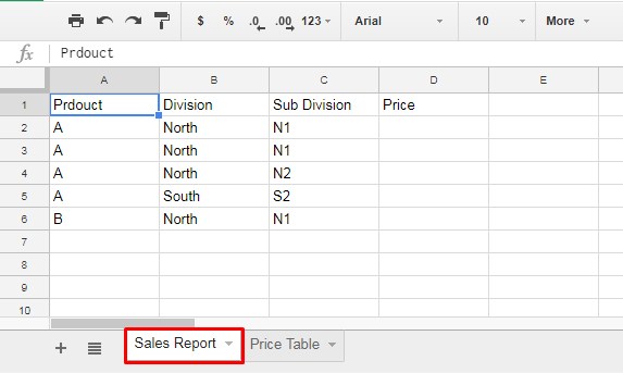
I intend to automatically populate the “Price” column when entering values under “Product,” “Division,” and “Sub Division.”

The pricing varies for each product and changes with alterations in “Division” and “Sub Division.”

I have a “Price Table” on another tab, as illustrated below.

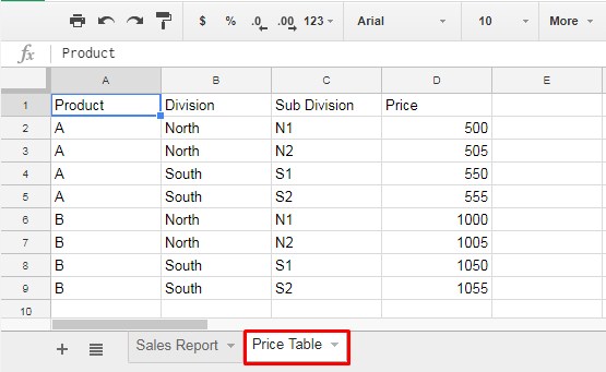
The objective is to populate the “Price” from this tab’s data onto the “Sales Report” tab, specifically under the “Price” column.

Achieving this necessitates comparing data in both sheets using a formula to obtain the desired results.

You can accomplish this task using a simple formula in Google Sheets. Follow the steps below to auto-populate values in cells based on conditions in Google Sheets.

Auto-Fill Cells with Matching Multiple Conditions Using the FILTER Function

Below is the formula for filling cells by matching multiple conditions in Google Sheets.

The formula should be entered in cell D2 in the “Sales Report” sheet, then copy and paste it into the cell right below to auto-populate the value.

=FILTER(
     'Price Table'!$D$2:$D, 
     'Price Table'!$A$2:$A=A2, 
     'Price Table'!$B$2:$B=B2, 
     'Price Table'!$C$2:$C=C2
)

Let me explain this formula, and then we’ll make it spill down from cell D2 without dragging it down.

This formula follows the FILTER function syntax:

FILTER(range, condition1, [condition2, …])

Where:

• range: ‘Price Table’!$D$2:$D
• condition1: ‘Price Table’!$A$2:$A=A2
• condition2: ‘Price Table’!$B$2:$B=B2
• condition3: ‘Price Table’!$C$2:$C=C2

The formula filters the price column in the ‘Price Table’ sheet, matching the product, division, and subdivision columns in that sheet with the corresponding values in cells A2, B2, and C2 in the ‘Sales Report’ sheet.

When dragging the formula down, A2, B2, and C2 become A3, B3, and C3, and so forth, and the corresponding prices are extracted.

How can we configure this formula to automatically fill cells based on multiple matching conditions?

How Can We Make This Formula Spill Down Starting from Cell D2?

The formula above doesn’t spill down automatically; instead, it requires manual dragging. To enable automatic expansion downward, use the MAP lambda function.

Within MAP, specify ranges A2:A, B2:B, and C2:C to iterate over values in these columns. Therefore, there’s no need to drag the formula from D2 down.

Formula:

=IFERROR(
     MAP(A2:A, B2:B, C2:C, LAMBDA(x, y, z, 
          FILTER(
               'Price Table'!$D$2:$D, 
               'Price Table'!$A$2:$A=x, 
               'Price Table'!$B$2:$B=y, 
               'Price Table'!$C$2:$C=z
          )
     ))
)

Let’s break down the formula step by step, starting with the syntax:

Syntax: MAP(array1, [array2, …], LAMBDA([name, …], formula_expression))

Here, A2:A, B2:B, and C2:C are array1, array2, and array3. The names to identify values in these arrays are x, y, z.

The formula_expression is the earlier FILTER formula, where A2 is replaced with x, B2 with y, and C2 with z for iteration over values in the arrays. IFERROR is employed to handle potential errors and return a blank result.

This array formula auto-fills cells with matching multiple conditions in Google Sheets.

Auto-Fill Cells with Matching Multiple Conditions Using the XLOOKUP Function

The XLOOKUP function searches for a search key in a column (lookup range) and returns a value from another column (result range). However, the challenge here is that we want to search for three keys in three columns and return a value from the price column.

To address this, we will combine the three columns into one and the three search keys into one.

You can enter this formula in cell D2 and drag it down:

=ArrayFormula(
     XLOOKUP(
          A2&B2&C2, 
          'Price Table'!$A$2:$A&'Price Table'!$B$2:$B&'Price Table'!$C$2:$C, 
          'Price Table'!$D$2:$D, 
          "'
     )
)

Syntax:

XLOOKUP(search_key, lookup_range, result_range, [missing_value], [match_mode], [search_mode])

Where:

• search_key: A2&B2&C2
• lookup_range: ‘Price Table’!$A$2:$A&’Price Table’!$B$2:$B&’Price Table’!$C$2:$C
• result_range: ‘Price Table’!$D$2:$D
• missing_value: “”

We have used ARRAYFORMULA as we combine columns, and that operation requires array formula support.

How do we expand it down?

Unlike FILTER, you do not need to use MAP or any other lambda function to expand this formula down. Simply replace A2&B2&C2 with A2:A&B2:B&C2:C:

=ArrayFormula(
     XLOOKUP(
          A2:A&B2:B&C2:C, 
          'Price Table'!A2:A&'Price Table'!B2:B&'Price Table'!C2:C, 
          'Price Table'!D2:D, 
          ""
     )
)

This is the XLOOKUP alternative to auto-fill cells with matching multiple values.

Resources

Above, I’ve provided two formula approaches to auto-fill cells with matching multiple values in Google Sheets. We can replace XLOOKUP with VLOOKUP and FILTER with QUERY as well.

However, the two formulas mentioned above should be sufficient to meet your requirements. Here are some resources related to auto-filling cells.

1. How to Autofill Alphabets in Google Sheets
2. Autofill Columns to the Right Based on the Value on the Left in Sheets
3. Auto-Fill Sequential Dates When Value Entered in Next Column in Google Sheets
4. Automatically Pre-fill Google Forms from Google Sheets: A Step-by-Step Guide
5. How to Autofill Days of the Week in Google Sheets