How to Use UNIQUE and SUM Together in Google Sheets

In certain situations, it’s important to know the use of UNIQUE and SUM together in Google Sheets.

Almost all spreadsheet users know the use of the UNIQUE function. It’s to return unique values from a range.

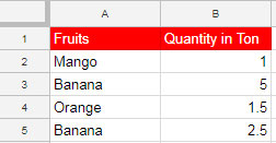
No matter what values, they can be text or numeric values. But there is a shortfall. See the below screenshot.

UNIQUE and SUM together in Google Sheets

Here what we want is, get the unique texts from column A and sum the corresponding values in column B against it.

Here you can apply the UNIQUE formula in two ways. But none can return our desired result.

Formula # 1

=unique(A2:B5)

There is no point in using the above formula as it would return the data as it’s.

As a side note, if you intend to unique the fruits column and return a two-column result, then try the following SORTN formula.

=sortn(A2:B5,9^9,2,1,1)

Formula # 2

=unique(A2:A5)

It has logic. But it only returns the unique value from column A. It won’t sum the values in column B.

So you should know how to use UNIQUE and SUM together in Google Sheets.

Steps to Combine UNIQUE and SUM together in Google Sheets

In the normal case, we can’t use SUM with UNIQUE to get the correct result.

We may require to use SUMIF in this case.

A Query formula is also workable. I’ll come to that part later.

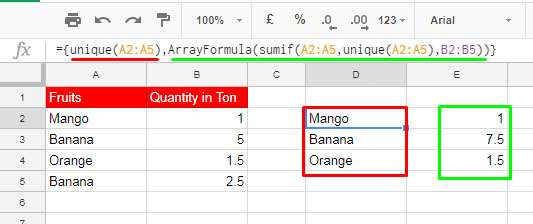
Here we are going to combine UNIQUE and SUMIF to get the result as below.

UNIQUE and SUMIF together in Google Sheets

Sumif and Unique Combo Formula:

={unique(A2:A5),ArrayFormula(sumif(A2:A5,unique(A2:A5),B2:B5))}

How to develop this combined UNIQUE and SUMIF Google Sheets formula? Let me explain it.

Earlier I’ve followed a similar approach. That time I have used a combined SUMIF formula to sum by month.

Once you complete this tutorial, please check that also here – Sum by Month in Google Sheets Using Combined SUMIF Formula. Now to the steps:

The following is the first part of the above combo formula. It’s a regular Unique formula to return the Unique texts from column A.

Formula 1:

=unique(A2:A5)

The second part is a SUMIF formula with a slight variation from its regular use.

Formula 2:

=sumif(A2:A5,unique(A2:A5),B2:B5)

To make you clearly understand this formula, I am going to compare it with the SUMIF syntax.

Syntax:

SUMIF(range,criterion,sum_range)

In the above formula # 2 part, Unique(A2:A5) returns multiple values as criteria.

So we should include ArrayFormula to cover all the criteria.

join UNIQUE and SUMIF together in Google Sheets

Finally, with the help of Curly Braces, I’ve combined Formula 1 and 2.

This way, you can use UNIQUE and SUM together in Google Sheets.

But there is an alternative to this formula. You can use a QUERY formula as below.

=query(A2:B5,"Select A, sum(B) group by A label Sum(B)''")

Thanks for the stay. Enjoy!

32 COMMENTS

Jessica Y August 29, 2023 At 11:59 pm

Prashanth,

Can you help me? I am trying to get a dataset to sum only unique values for a certain date.

Date (A) | Weight (B)
2023-08-23 | 1487
2023-08-23 | 1487
2023-08-23 | 1487
2023-08-23 | 1487
2023-08-23 | 1462
2023-08-23 | 1462
2023-08-23 | 1462
2023-08-23 | 1462
2023-08-23 | 1431
2023-08-23 | 1431
2023-08-23 | 1431
2023-08-23 | 1431

The current formula is:

=SUMIFS(B:B, A:A, G2, B:B, UNIQUE(B:B))

It sums the column by date when A:A is equal to G2 and B:B is unique. However, it keeps returning 0.

- Prashanth August 31, 2023 At 10:01 am
  
  Hi Jessica Y,
  
  You can use a combination of the SUM, UNIQUE, and FILTER functions as follows.
  
  =SUM(UNIQUE(FILTER(B:B,A:A=G2)))
  
NS January 31, 2023 At 11:41 am

Hi,

I’m facing an issue with three columns.

Here is a sample data set:

Name | Tickets | Department
Joe | 2 | Security
Tia | 3 | Reception
Joe | 4 | Security

Expected output:

Name | Tickets | Department
Joe | 6 | Security
Tia | 3 | Reception

I tried the Query you shared, and it works for 1 column and sum, but I am facing an issue in displaying multiple columns.

Any help is appreciated.

Thanks
– NS

- Prashanth February 2, 2023 At 1:34 pm
  
  Hi, NS,
  
  You are on the right track. Use the QUERY() as below.
  
  =query(A1:C,"Select A,sum(B),C where A is not null group by A,C label sum(B)'Tickets'",1)
  
Frosty January 19, 2023 At 2:02 am

Thank you!

Frosty January 9, 2023 At 11:27 pm

Prashanth,

I do have a question after all. I can’t figure out the formula when working with 3 columns of data, and I also need to ignore blank cells.

Example:

I want to unique sum column C based on columns A and B. I want to know how many jobs John Doe has Completed and the total amount for all completed jobs. I also want to ignore blank cells in column A. I also want to know how many jobs John Doe has “In Progress” and the total amount.

After that, I will use a simple =query(A:A, "Order by DESC") for an employee ranking system.

I am working with live data that auto-populates every 1min.

- Prashanth January 11, 2023 At 9:24 am
  
  Hi, Frosty,
  
  The following formula might help.
  
  =query(A2:C,"Select A,count(C),sum(C) where A='John Doe' and B='Completed' group by A,B")
  
  Next, replace ‘Completed’ with ‘In Progress’
  
  If you have any issue implementing the same, please feel free to share a sample Sheet (URL in your reply)
  
  The following tutorial might help you progress in the popular QUERY function in Google Sheets.
  
  What is the Correct Clause Order in Google Sheets Query?
  
  Update:-
  
  The following formula is for Unique and Sum every employee and to sort the sum column too.
  
  =query(A2:C,"Select A,count(C),sum(C) where A is not null and B='Completed' group by A,B order by sum(C) desc,A asc")
  
  - Frosty January 11, 2023 At 9:40 pm
    
    Prashanth! I can not thank you enough! It works and is precisely what I needed. You even took it a step further with the desc and asc! Thank you!
    
    I do have one more question. The formula spits out count and sum text. Can I stop this or change the text the formula is producing?
    
    - Prashanth January 13, 2023 At 5:23 pm
      
      Hi, Frosty,
      
      You require to use the QUERY LABEL clause.
      
      =query(A2:C,"Select A,count(C),sum(C) where A='John Doe' and B='Completed' group by A,B label count(C)'',sum(C)''")
      
      I hope that help.
      
Scott Frost January 9, 2023 At 10:57 pm

I am working with live data that auto-populates. This formula is perfect, but I need it to ignore bank cells. Any chance it can do that?

Thank you,

-Scott

- Frosty January 9, 2023 At 11:03 pm
  
  Never mind! I figured it out!
  
  - Prashanth January 11, 2023 At 9:11 am
    
    Hi, Frosty,
    
    It’s nice to hear that you found a solution to it.
    
    Even so, here are my suggestions for other users.
    
    When using Query()
    
    ={unique(A2:A),ArrayFormula(sumif(A2:A,unique(A2:A),B2:B))}
    
    When using Sumif()
    
    =ArrayFormula({unique(filter(A2:A,len(A2:A))), sumif(A2:A,unique(filter(A2:A,len(A2:A))),B2:B)})
    
CT November 16, 2022 At 2:50 am

Hi! I used your formula ={unique(A2:A5),ArrayFormula(sumif(A2:A5,unique(A2:A5),B2:B5))} successfully.

I’m trying to alter the criteria a bit to look at unique information from A2:A5 + specific information from column B: B2:B5, “Y”.

I keep getting an error when trying to incorporate it into this formula. Are you able to help?

- Prashanth November 16, 2022 At 9:20 am
  
  Hi, CT,
  
  You may better use a QUERY.
  
  Use the following formula when the group column is A, the criteria column is B, and the sum column is C.
  
  =query(A2:C,"Select A,sum(C) where lower(B)='y' group by A label sum(C)''")
  
matt August 2, 2022 At 11:53 pm

Hi,

I used your formula (thank you!) for a list where there are some blanks.

Can you show me how to eliminate blanks from showing up in the array outcome?

={unique(D6:D35),ArrayFormula(sumif(D6:D35,unique(D6:D35),E6:E35))}

- Prashanth August 3, 2022 At 11:37 am
  
  Hi, matt,
  
  Include Filter as below.
  
  =ArrayFormula({unique(filter(D6:D35,len(D6:D35))), sumif(D6:D35,unique(filter(D6:D35,len(D6:D35))),E6:E35)})
  
Nathan Rayle July 14, 2022 At 12:33 am

Hi, thank you for this post.

I’m attempting to get the sum of unique values (Col B) that have “<2.5" (Col F) in the term "F1" (Col E).

I have this formula:

=SUMIFS(F:F,F:F,”< 2.5",E:E,"F1")

And it gives the total of all grades with a Term of “F1” below 2.5.

Now, I need only to count each unique value 1x, to get the total number of students who have at least 1 grade below a 2.5 in “F1”.

Thank you.

- Prashanth July 14, 2022 At 9:28 am
  
  Hi, Nathan Rayle,
  
  I’m not clear about the last part of your query, i.e., “Now, I need…”
  
  Can you share the URL of your Sheet (sample) in your reply below?
  
Danielle S March 12, 2022 At 2:24 am

This is great! what’s the workaround if your original data does not match the same case? i.e., Banana or banana but I want them to show up as the same item count.

- Prashanth March 13, 2022 At 10:58 am
  
  Hi, Danielle S,
  
  Use UPPER or LOWER within QUERY()
  
  When the range is A2:B5.
  
  =query(A2:B5,"Select Upper(A), sum(B) group by Upper(A) label Upper(A)'',Sum(B)''")
  
  When you use an open range such as (A2:B).
  
  =query(A2:B,"Select Upper(A), sum(B) where A is not null group by Upper(A) label Upper(A)'',Sum(B)''")
  
Kris October 8, 2021 At 1:46 am

Thank you for your time.

I have a job list that includes a lot of information per job, including wood types and colors used.

I have a list (without duplicates) using sort, unique, filter, and flatten functions.

I would like to add how many times each wood type and/or color is used.

Any help is appreciated.

- Prashanth October 8, 2021 At 12:47 pm
  
  Hi, Kris,
  
  You may use Query().
  
  If you share a sample, I will try to help you solve it. You can leave the address (Sheet URL) below.
  
Mr. A July 23, 2021 At 2:13 pm

Thanks so much for your help. Quick question, would you know if there is a way of using this Unique and Sumif array formula you’ve explained while sorting the numerical values from largest to smallest?

Kind regards,
Mr. A

- Prashanth July 25, 2021 At 10:41 am
  
  Hi, Mr. A,
  
  Include SORT as below.
  
  =SORT({unique(A2:A5),sumif(A2:A5,unique(A2:A5),B2:B5)},2,0)
  
  Note:- Removed the ArrayFormula as the SORT takes care of the role.
  
Janice Lane July 8, 2021 At 12:46 am

I am trying to get a total of one column and only including the unique entries from another column. I am getting an error message stating formula parse error.

This is the formula I am using.

={unique(D5:D800), ArrayFormula(sumif(D5:D800, unique(D5:D800), K5:K800)}

What do I need to do to correct this?

- Prashanth July 8, 2021 At 10:08 am
  
  Hi, Janice Lane,
  
  Try this instead. You were missing one closing bracket before the last curly bracket.
  
  ={unique(D5:D800), ArrayFormula(sumif(D5:D800, unique(D5:D800), K5:K800))}
  
Norman Navarro May 13, 2021 At 8:46 am

This is great, can I ask how I would bring the first column and the total entries for each? I am trying to get UNIQUE and COUNTIF to work together.

- Prashanth May 13, 2021 At 9:14 am
  
  Hi, Norman Navarro,
  
  You may simply try the below Query.
  
  =query(A1:A,"Select A,count(A) where A is not null group by A",1)
  
  If the range A1:A doesn’t have the header row (label in A1), then use 0 instead of 1 in the last part of the above Query.
  
Nick November 16, 2020 At 9:23 am

I am trying to do exactly this, but only return the sums without the first column:

I got {ArrayFormula(sumif(ExpensesDB!A2:A,unique(ExpensesDB!A2:A),ExpensesDB!C2:C))} but this didn’t combine all of the common month numbers it just returned everything from Column A.

- Prashanth November 16, 2020 At 10:13 am
  
  Hi, Nick,
  
  You can try this.
  
  ={unique(ExpensesDB!A2:A), ArrayFormula(sumif(ExpensesDB!A2:A,unique(ExpensesDB!A2:A), ExpensesDB!C2:C))}
  
  Here is another tutorial in line with the above.
  
  Sum by Month in Google Sheets Using Combined SUMIF Formula
  
Hector March 25, 2019 At 8:18 pm

I am trying to create this arrangement but bringing the information from a second sheet ( in the same file) but does not work this formula.

Do you know why?

- Prashanth March 26, 2019 At 8:08 am
  
  Please share an example sheet.