The SUMIF function is useful for conditional sums in Google Sheets. But do you know how to use SUMIF while excluding hidden rows in Google Sheets?

The Google Sheets SUBTOTAL function can help you deal with hidden rows, but it may not accept criteria or conditions. So, I am aiming for a combination of SUMIF and SUBTOTAL. But is that even possible? Let’s find out.

Can We Use the SUMIF Function Only on Visible Rows?

The answer is no. You should switch to the SUMIFS function instead.

Why SUMIFS?

To specify hidden rows, we need an additional criteria range that contains SUBTOTAL. SUMIF won’t support this, but SUMIFS does, as it can handle multiple criteria ranges and criteria.

There are two methods we can adopt to use SUMIFS for visible rows: one uses a physical helper column, and the other does not use a physical helper column.

Excluding Hidden Rows in SUMIFS Using a Physical Helper Column

Let’s begin with how to apply conditional sum excluding hidden rows.

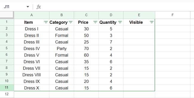
Our actual sample data is spread across the range A1:D11 where A1:D1 contains the field labels. In cell E1, enter the field label for the helper column; I am inputting ‘Visible’. You can enter your choice of label.

Let’s apply a filter to this table. There are two approaches. You can either select the range and apply Data > Create a filter or select the range and apply Format > Convert to a table. I am following the former one.

Steps to Create the Helper Column

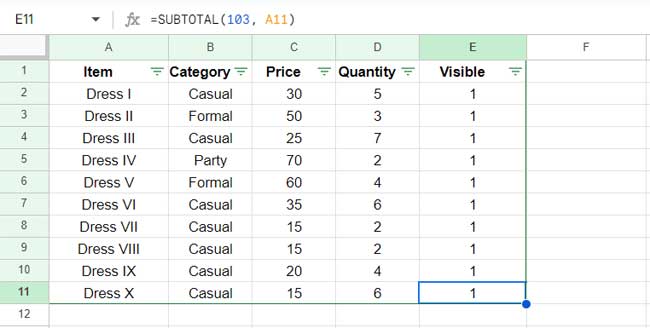
In cell E2, enter the following formula that returns the count of value in cell A2:

=SUBTOTAL(103, A2)

This returns the count of value irrespective of number or text. The function number 103 represents counta in SUBTOTAL.

Drag down the fill handle of E2 to E11, and the helper column for SUMIFS in visible rows is ready.

The formula will return 1 in all visible rows in E2:E11; the value will be 0 when hidden.

Important:

The formula counts the value in cell A2. Why this cell reference?

This is because we’re using SUBTOTAL to count visible rows, and blank cells in the chosen column might lead to inaccurate counts. You can refer to the first row in any column in the range that doesn’t contain a blank cell.

Another thing is the function number used in the formula, which is 103. It excludes all types of hidden rows:

• Rows filtered through Data > Create a filter, Insert > Tables, Data > Add a slicer; collectively known as Filtering.
• Rows made hidden via right-click context menu “Hide rows” or View > Group > Group rows; collectively known as Hidden.

If you are specific to “Filtering” only, use the function number 3 instead.

Formula Examples

Assume you want to get the total quantity of Casual wear. You can use either of the following SUMIF or SUMIFS formulas without considering the visibility of rows:

=SUMIF(B2:B11, "Casual", D2:D11)

As per the syntax: SUMIF(range, criterion, [sum_range])

=SUMIFS(D2:D11, B2:B11, "Casual")

As per the syntax: SUMIFS(sum_range, criteria_range1, criterion1, [criteria_range2, …], [criterion2, …])

When you filter any column, the formula will return the same result, as they are not ready to handle the hidden rows.

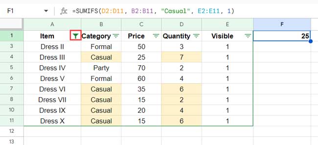
Here is how to use the SUMIFS formula in visible rows, meaning exclude hidden rows in the calculation:

=SUMIFS(D2:D11, B2:B11, "Casual", E2:E11, 1)

When you filter out any row, for example, “Dress I” and “Dress XIII” in column A, the formula will exclude those rows in the calculation.

You can filter any column in the range, and the formula will exclude those rows.

Excluding Hidden Rows in SUMIFS Without Using a Physical Helper Column

We can’t exclude hidden rows in SUMIF. So we used SUMIFS with a helper column. However, the above helper column approach is non-dynamic due to the following reasons:

1. When you add new records (new rows in the range), you’ll need to ensure that SUBTOTAL formulas are added to the newly added rows.
2. It requires an extra column which might not be ideal for some users.

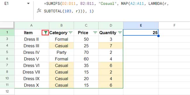
We can address both issues by replacing E2:E11, the helper range reference in the SUMIFS excluding hidden rows, with the following MAP formula:

MAP(A2:A11, LAMBDA(r, SUBTOTAL(103, r)))

So the formula will become:

=SUMIFS(D2:D11, B2:B11, "Casual", MAP(A2:A11, LAMBDA(r, SUBTOTAL(103, r))), 1)

Let me explain the MAP section:

In the physical helper column approach, the formula in E2 was SUBTOTAL(103, A2). Here we converted it to a custom lambda function as LAMBDA(r, SUBTOTAL(103, r)) where r represents the current element in the array.

We need to specify the array A2:A11 in MAP so that the custom function will return the SUBTOTAL output in each row in the array. The MAP function iterates through r for each value in the array.

This enables us to use the MAP formula instead of the helper column E2:E11 in the SUMIFS.

Resources

• Find the Average of Visible Rows in Google Sheets
• Count Unique Values in Visible Rows in Google Sheets
• IMPORTRANGE to Import Visible Rows in Google Sheets
• XLOOKUP Visible (Filtered) Data in Google Sheets
• XMATCH Visible Rows in Google Sheets
• Weighted Average of Filtered (Visible) Data in Google Sheets
• UNIQUE Function in Visible Rows in Google Sheets
• How to Omit Hidden or Filtered Out Values in Sum
• Google Sheets Query Hidden Row Handling with Virtual Helper Column
• Vlookup Skips Hidden Rows in Google Sheets – Formula Example
• Insert Sequential Numbers Skipping Hidden | Filtered Rows in Google Sheets
• COUNTIF | COUNTIFS Excluding Hidden Rows in Google Sheets