This tutorial is for users who want to apply XLOOKUP inside a structured table in Google Sheets (created via Insert > Table or Convert range to table). You’ll learn how to use both single and multiple conditions with structured references across two tables:
- A main (primary) table, where the formula is written.
- A lookup (reference) table, where the data is retrieved from.
Using structured references can make formulas cleaner and easier to manage—especially inside tables.
What Is “XLOOKUP Inside a Structured Table Row”?
It means writing an XLOOKUP formula that refers to structured column names within a table row, instead of traditional range references like A2:A10. This approach:
- Auto-expands to new rows (like Excel tables).
- Keeps formulas dynamic and readable.
- Supports both simple and multi-condition lookups.
Single Condition XLOOKUP in a Structured Table (Google Sheets Example)
Goal: Return the employee’s role from the lookup table based on the employee ID in the main table using structured references.
Table Structure:
Lookup Table (Table1):
| Employee ID | Role |
|---|---|
| EMP001 | Sales Associate |
| EMP002 | HR Manager |
| EMP003 | Software Engineer |
| EMP004 | Data Analyst |
| EMP005 | Marketing Lead |
Main Table (Table2):
| Employee ID | Role |
|---|---|
| EMP001 |
Formula in Table2[Role]:
=XLOOKUP(SINGLE(Table2[Employee ID]), Table1[Employee ID], Table1[Role])- The
SINGLE()function ensures only one value is passed toXLOOKUP. - The result auto-fills as new rows are added next to the last row.
Note: If you use the + (plus) button to insert a new row, the formula won’t auto-copy. Instead, type directly next to the last value.
ARRAYFORMULA with XLOOKUP in a Structured Table
If you prefer one formula that covers the entire column:
=ARRAYFORMULA(XLOOKUP(Table2[Employee ID], Table1[Employee ID], Table1[Role]))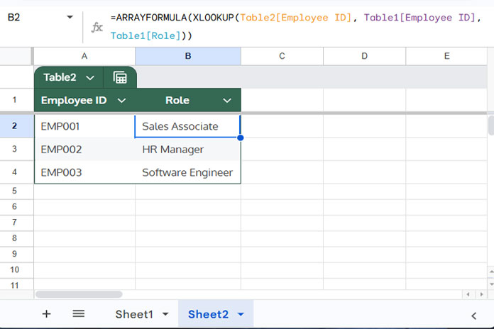
Multi-Condition XLOOKUP in Google Sheets Using Structured References
Goal: Return the product price by matching item, size, and color across two structured tables using multiple-condition XLOOKUP.
Table Structure:
Lookup Table (Table1):
| Employee ID | Role |
|---|---|
| EMP001 | Sales Associate |
| EMP002 | HR Manager |
| EMP003 | Software Engineer |
| EMP004 | Data Analyst |
| EMP005 | Marketing Lead |
Main Table (Table2):
| Item | Size | Color | Price |
|---|---|---|---|
| T-shirt | M | Red |
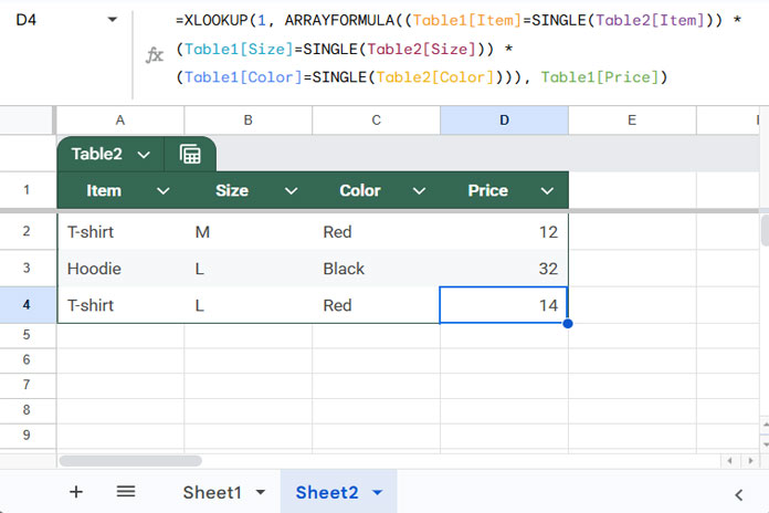
Formula (for one row):
=XLOOKUP(1, ARRAYFORMULA((Table1[Item]=SINGLE(Table2[Item])) * (Table1[Size]=SINGLE(Table2[Size])) * (Table1[Color]=SINGLE(Table2[Color]))), Table1[Price])Explanation:
- Each condition returns TRUE (1) or FALSE (0).
- All TRUEs multiply to 1.
XLOOKUPsearches for1and returns the corresponding price.
Array Formula for Multi-Condition XLOOKUP in Google Sheets
To make it work across all rows in Table2:
=MAP(Table2[Item], Table2[Size], Table2[Color], LAMBDA(x, y, z, XLOOKUP(1, ARRAYFORMULA((Table1[Item]=SINGLE(x)) * (Table1[Size]=SINGLE(y)) * (Table1[Color]=SINGLE(z))), Table1[Price])))MAPiterates over each row.LAMBDAcreates dynamic row-based XLOOKUP logic.
Alternative Method for Multi-Criteria XLOOKUP (Using Text Join)
You could combine the lookup conditions using & and search a concatenated column:
=ARRAYFORMULA(XLOOKUP(Table2[Item]&Table2[Size]&Table2[Color], Table1[Item]&Table1[Size]&Table1[Color], Table1[Price]))Summary
In this tutorial, you learned how to use XLOOKUP inside a structured table in Google Sheets, both for single-condition and multiple-condition lookups. With structured references and dynamic array formulas like ARRAYFORMULA and MAP, your lookups stay clean, scalable, and easy to manage.
If you want to explore more techniques like this, visit our Complete Guide to XLOOKUP in Google Sheets, where we compile practical XLOOKUP examples in Google Sheets ranging from beginner formulas to advanced lookup strategies.


