How to Get the Fastest Time for Each Person in Google Sheets

Whether you’re tracking race results, event times, or any other timed activities, finding the best (shortest) time for each individual helps you quickly summarize the results. In this guide, we’ll show you how to group names and return the fastest time for each person using simple formulas in Google Sheets.

Table of Contents

Preparing the Data

To find the shortest time per name in Google Sheets, it’s important to organize your data in a specific way with four columns:

First name
Last name
Minutes
Seconds (which may include milliseconds)

While combining the first and last names, as well as combining the minutes and seconds, can simplify the formula, I prefer working with the four-column format. This structure adds complexity to the formula, as it involves combining the minutes and seconds, but it provides a more adaptable approach when coding the solution.

Sample Data to Find the Shortest Time Per Person

First Name	Last Name	Min	Sec
Adam	Kidd	2	0.8
Adam	Kidd	1	58.45
Victoria	Lopez	2	4.51
Bobbie	Castillo	2	9.11
Bobbie	Castillo	2	13.22
Olga	Ashley	2	36.85
Olga	Ashley	2	45.8
Cary	Hansen	2	28.56
Cary	Hansen	2	30.17

Do I Need to Sort the Table?

No. You don’t need to sort the table by name, time, or any other field. The formula will handle everything for you, including sorting names and times automatically.

Formula to Get the Fastest Time for Each Person in Google Sheets

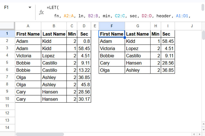
In this setup, with your data in columns A1:D (where A1:D1 contains field labels), you can use the following formula in cell F1:

=LET(
   fn, A2:A, ln, B2:B, min, C2:C, sec, D2:D, header, A1:D1, 
   table, SORT(HSTACK(HSTACK(fn, ln, min, sec), (min * 60 + sec) / 86400, fn&ln), 6, 1, 5, 1), 
   fnl, CHOOSECOLS(SORT(SORTN(FILTER(table, CHOOSECOLS(table, 1)<>""), 9^9, 2, 6, 1), 5, 1), 1, 2, 3, 4), 
   VSTACK(header, fnl)
)

This formula processes the range A1:D and returns the fastest time for each person as follows:

Example of how to get the fastest time for each person in Google Sheets

Anatomy of the Formula

There are a couple of components in the formula.

First, we assign names to each column and the header as follows:

fn, A2:A, ln, B2:B, min, C2:C, sec, D2:D, header, A1:D1

This makes the formula easily adaptable to different ranges.

Then, we process the range A2:D:

table, SORT(HSTACK(HSTACK(fn, ln, min, sec), (min * 60 + sec) / 86400, fn&ln), 6, 1, 5, 1)

This returns A2:D and appends two more columns: one with the combined minutes and seconds, and another with the combined first and last names. It then sorts by the combined columns, placing the names in ascending order. If the name repeats, the fastest time will be at the top.

Finally, the next part removes duplicate names and ensures we get the shortest time for each person:

fnl, CHOOSECOLS(SORT(SORTN(FILTER(table, CHOOSECOLS(table, 1)<>""), 9^9, 2, 6, 1), 5, 1), 1, 2, 3, 4)

This part uses the SORTN fun c tion to remove duplicates, ensuring each person only has their fastest time listed. The SORT function sorts the data by time, arranging names by their fastest times.

VSTACK(header, fnl) simply adds the header row to the result.

And that’s how you get the fastest time for each person!

Filter and Display the Top 3 Fastest Times in Google Sheets

Once you’ve filtered the fastest time for each person, you may want to focus on just the top 3 fastest overall times. This can help you quickly identify the best performances without having to sift through a long list of results. In this section, we’ll show you how to filter and display only the top 3 fastest times in your dataset, ensuring you get the most relevant data at a glance.

To achieve this, you can incorporate the ARRAY_CONSTRAIN function into the formula.

Simply replace ‘fnl’ in VSTACK(header, fnl) with ARRAY_CONSTRAIN(fnl, 3, 4).

The updated formula will look like this:

=LET(
   fn, A2:A, ln, B2:B, min, C2:C, sec, D2:D, header, A1:D1, 
   table, SORT(HSTACK(HSTACK(fn, ln, min, sec), (min * 60 + sec) / 86400, fn&ln), 6, 1, 5, 1), 
   fnl, CHOOSECOLS(SORT(SORTN(FILTER(table, CHOOSECOLS(table, 1)<>""), 9^9, 2, 6, 1), 5, 1), 1, 2, 3, 4), 
   VSTACK(header, ARRAY_CONSTRAIN(fnl, 3, 4))
)

This will display only the top 3 fastest times in your dataset.

Sample Sheet