Want to track progress over time? In this tutorial, I’ll show you how to calculate elapsed percentage between dates in Google Sheets. This helps you monitor the progress of tasks, projects, or timelines by showing how much of the time between a start and end date has passed—automatically and accurately.
There are essentially three dates involved: a start date, an end date, and another reference date, which can be today’s date or a specific target date.
For example, if a task starts on 01 May 2025 and ends on 31 May 2025, you can calculate how much time has elapsed as of today or any point in time, such as 20 May 2025.
Formula to Calculate Elapsed Percentage Between Dates in Google Sheets
=LET(
   start, DATEVALUE(A2), end, DATEVALUE(B2), target, $D$1,
   duration, IFERROR(MAX(0, DAYS(end, start)+1)),
   elapsed, IFERROR(MAX(0, DAYS(IF(end>=target, target, end+1), start))),
   TO_PERCENT(elapsed/duration)
)- The formula assumes the start date is in cell
A2, the end date is inB2, and the reference date (e.g. today’s date) is inD1. - Both the start and end dates are treated as inclusive.
Formula Explanation
DATEVALUE: Ensures blank cells don’t default to 30/12/1899, which would otherwise skew the results.IFERROR(MAX(0, DAYS(end, start) + 1)): Calculates the total duration between start and end dates, including both.IFERROR(MAX(0, DAYS(IF(end >= target, target, end + 1), start))): Calculates the elapsed number of days up to the reference date.TO_PERCENT(elapsed / duration): Converts the fraction into a percentage—this is your elapsed percentage between dates.
Example: Calculating Elapsed Percentage Between Dates in Google Sheets
Assume your project start dates are in column A2:A and end dates in B2:B.
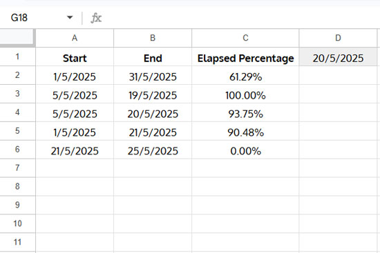
- In cell D1, enter:
=TODAY() - In cell C2, enter the formula:
=LET(
   start, DATEVALUE(A2), end, DATEVALUE(B2), target, $D$1,
   duration, IFERROR(MAX(0, DAYS(end, start)+1)),
   elapsed, IFERROR(MAX(0, DAYS(IF(end>=target, target, end+1), start))),
   TO_PERCENT(elapsed/duration)
) - Drag it down the column as needed.
Can I Apply This as an Array Formula?
Nope! Simply replacing A2 with A2:A and B2 with B2:B and entering it as an array formula won’t work. That’s because the MAX function doesn’t support array expansion in this context.
The workaround? Convert the formula into a custom LAMBDA function and use the MAP helper function to apply it across the ranges.
In cell C2, enter this version instead:
=MAP(
   A2:A, B2:B,
   LAMBDA(start_dt, end_dt,
      LET(
         start, DATEVALUE(start_dt), end, DATEVALUE(end_dt), target, $D$1,
         duration, IFERROR(MAX(0, DAYS(end, start)+1)),
         elapsed, IFERROR(MAX(0, DAYS(IF(end>=target, target, end+1), start))),
         TO_PERCENT(IFERROR(elapsed/duration))
      )
   )
)
This formula will calculate the elapsed percentage between dates in Google Sheets for each row in your dataset.
FAQs: Elapsed Percentage Between Dates in Google Sheets
How do I calculate the percentage of time elapsed between two dates in Google Sheets?
First, cap the dates so they don’t go beyond the start or end dates. Then, calculate the elapsed days and total duration, and divide the elapsed by the duration to get the percentage.
Can I track progress automatically with today’s date?
Yes. By using TODAY() as the reference date, your formula will update daily and show the real-time progress between the given dates.
What happens if the reference date is after the end date?
The formula caps the reference date to the end date, ensuring the elapsed percentage does not exceed 100%.
Can I use this formula for multiple rows?
Yes, by using the MAP and LAMBDA functions, you can apply the elapsed percentage calculation across entire columns.


