Calculating the number of days ignoring blank cells in Google Sheets is a common task when working with dates for payrolls, project timelines, or attendance tracking. Built-in functions like DAYS, DATEDIF, NETWORKDAYS, and NETWORKDAYS.INTL don’t handle blank cells properly. If a cell is empty, these functions can return very large positive or negative numbers, or even #NUM! errors, making your calculations unreliable.
In this guide, we’ll show you how to safely calculate days and network days while ignoring blank cells, using both simple and array-friendly formulas.
Why Blank Cells Cause Errors When Calculating Days in Google Sheets
Google Sheets stores dates as serial numbers:
0 = 30/12/18991 = 31/12/1899
Blank cells are treated as 0 internally.
Here’s an example of incorrect results when blank cells are not handled properly:
| Start Date | End Date | Formula | Result |
| 01/08/2025 | 05/08/2025 | =DAYS(B2, A2) | 4 |
| 02/08/2025 | =DAYS(B3, A3) | -45871 | |
| 06/08/2025 | =DAYS(B4, A4) | 45875 | |
| 03/08/2025 | 10/08/2025 | =DAYS(B5, A5) | 7 |
This clearly shows why handling blank cells is essential for accurate day calculations.
Solution 1: Using ISDATE to Calculate Number of Days Ignoring Blank Cells
The ISDATE function checks whether a cell contains a valid date. Combined with IF, it allows you to skip blank cells:
Non-Array Example Formula:
=IF(AND(ISDATE(A2), ISDATE(B2)), DAYS(B2, A2), )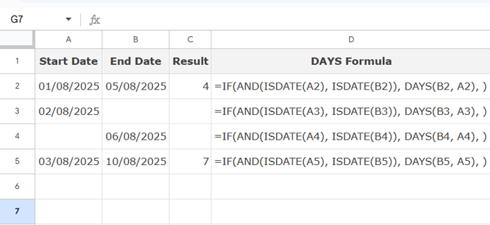
Other formulas using ISDATE include:
C2: =IF(AND(ISDATE(A2), ISDATE(B2)), NETWORKDAYS(A2, B2), )D2: =IF(AND(ISDATE(A2), ISDATE(B2)), NETWORKDAYS.INTL(A2, B2, 1), )E2: =IF(AND(ISDATE(A2), ISDATE(B2)), DATEDIF(A2, B2, "D"), )
These formulas return a blank if either the start or end date is missing.
Note: To learn more about the functions used above, including DAYS, DATEDIF, NETWORKDAYS, and NETWORKDAYS.INTL, please check Google Sheets: The Complete Guide to All Date Functions.
Solution 2: Using DATEVALUE + IFERROR
DATEVALUE converts a date or a date string into its corresponding numeric serial number in Google Sheets. Blank or invalid cells return #VALUE!, so wrapping it with IFERROR ensures the formula doesn’t break.
Non-Array Example:
=IFERROR(DAYS(DATEVALUE(B2), DATEVALUE(A2)))Array Formula to Calculate Number of Days Ignoring Blank Cells
To automatically apply the formula across multiple rows, you can use:
=ArrayFormula(IFERROR(DAYS(DATEVALUE(B2:B), DATEVALUE(A2:A))))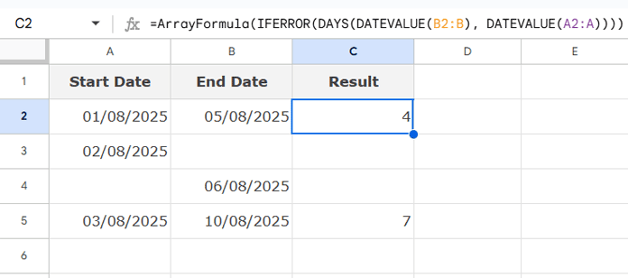
Advantages:
- Works with
DAYS,DATEDIF,NETWORKDAYS, andNETWORKDAYS.INTL - Auto-fills the entire column
- Handles blank cells without producing errors or huge numbers
Important Note:
The ISDATE function combined with AND does not work in array formulas:
ANDcan evaluate multiple values at once, but it returns a single TRUE if all values are TRUE, or FALSE otherwise. It cannot return individual TRUE/FALSE results for each element in an array.- When you refer
ISDATEto an array of cells (e.g.,ISDATE(A2:A)), it returns a single TRUE or FALSE, not an array of results for each row.
Because of this, using ISDATE + AND directly in an array formula will not produce correct per-row results.
If you want to retain the ISDATE logic in an array context, you can use LAMBDA with MAP:
=MAP(A2:A, B2:B, LAMBDA(start, end, IF(AND(ISDATE(start), ISDATE(end)), DAYS(end, start), )))- Evaluates each row individually
- Returns blank if either start or end date is invalid or missing
Summary
Blank date cells in Google Sheets can produce incorrect or unexpectedly large numbers in date calculations. To calculate the number of days ignoring blank cells in Google Sheets, you can:
- Use
ISDATEin non-array formulas - Use
DATEVALUEcombined withIFERRORin array formulas - Use
ARRAYFORMULAto automatically apply the formula across a column - Use
MAP + LAMBDAto replicate row-by-row logic if needed
These methods ensure accurate day and network day calculations, even when some date cells are blank.
Related Resources
- Find Number of Working and Non-Working Days in Google Sheets
- Elapsed Days and Time Between Two Dates in Google Sheets
- Add or Subtract Days from Dates in Google Sheets QUERY (2 Easy Methods)
- How to Calculate Days Since Last Payment in Google Sheets (Array Formula)
- Convert Month Name to Days in Google Sheets
- Task Duration, Remaining, and Elapsed Days Calculation: Google Sheets
- Calculate Trip Days by Month (Start, End, and Full Days) in Google Sheets


