First of all, let me clarify that we can use named ranges in conditional formatting using INDIRECT in Google Sheets. Before delving into an example, let’s explore some of the benefits of utilizing it in conditional formatting.
The most significant advantage is that the named ranges enhance the readability and understanding of your highlight rules. When you write a formula for other users or in a collaborative sheet, they can easily comprehend the formula.
If you rely on cell references, users may need to inspect the content in the cell/range references to grasp the formula. It is crucial to use meaningful names when assigning ranges.
Another advantage is that coding rules become more manageable because you won’t lose momentum when dealing with lengthy formulas.
But that doesn’t mean there are no drawbacks. Some drawbacks come to my immediate attention, which I have pointed out at the end of the tutorial. You can understand them once you have gone through all the examples below.
Examples of Using Named Ranges in Conditional Formatting
Here are a few examples of using named ranges in conditional formatting in Google Sheets. Once you have gone through these examples, you will become proficient in utilizing them in Google Sheets.
The first example highlights a cell range based on a named range. The other two examples highlight the named range itself. I’ve tried to bring some diversification in choosing the examples.
a. Match Values in the Named Range and Highlight
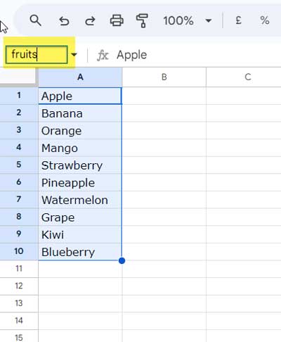
In the first example, we will name the range A1:A10 with the name “fruits” and highlight all the fruits in column E that are present in the named range. Please pay attention to assigning the name, as in the later examples, I won’t explain those steps again.
Steps:
Select the cell range A1:A10.
Click within the name box (the field left to the formula bar) and type “fruits,” then hit enter. Alternatively, go to Data > Named ranges and enter the name.
Go to Format > Conditional formatting and enter the range to highlight below “Apply to range.” Here, enter E1:E.
Below that, under “Format rules,” select “Custom formula is” and enter the following formula:
=MATCH(E1, INDIRECT("fruits"), FALSE)>0Click Done.
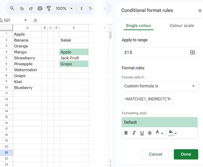
That’s it. All the values in column E that are present in fruits will be highlighted.
How does the usage of named ranges in conditional formatting differ from that of cell usage?
In regular formulas, you can use the named range as it is, whereas in conditional formatting, you should use it within the INDIRECT function as a string.
In the above example, we have used INDIRECT("fruits"), whereas in a regular formula, you can use it as fruits.
b. Highlight Values within the Named Range Area
In this example, we have a list of dates in B2:B7, named as holidays.
The objective is to highlight any holiday that falls on today or tomorrow. How do we achieve this using the named range holidays in the highlight rule for conditional formatting?
Here is the highlight rule (formula) to use in the custom formula rule for the apply-to range B2:B7:
=OR(INDIRECT("holidays")=TODAY(), INDIRECT("holidays")=TODAY()+1)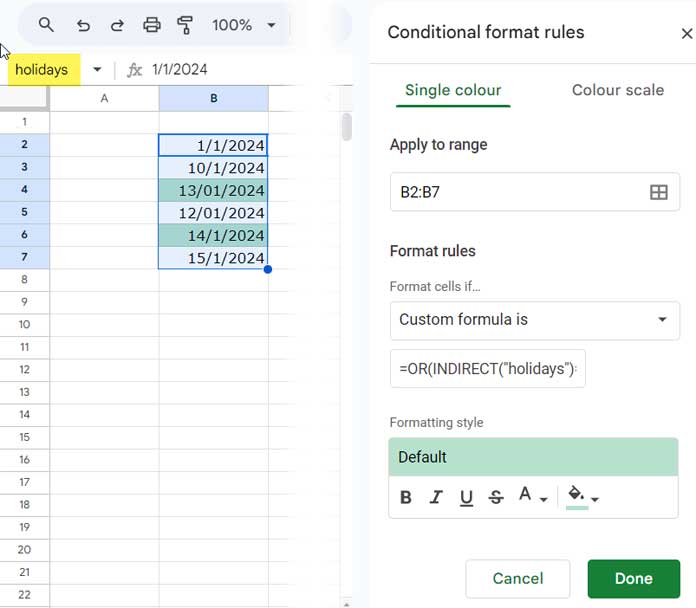
We have used an OR logical test to determine whether the dates in holidays match TODAY() OR TODAY()+1.
c. How to Use Named Ranges in Conditional Formatting to Highlight Duplicates within that Range
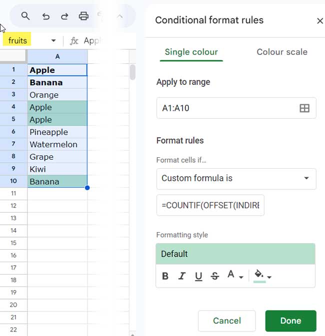
In our first example, we used the named range fruits for the range A1:A10. Let’s employ it for this example as well.
To highlight duplicates within a named range, we need to utilize the OFFSET function.
Formula Rule:
=COUNTIF(OFFSET(INDIRECT("fruits"), 0, 0, ROW(A1)), OFFSET(INDIRECT("fruits"), ROW(A1)-1, 0, 1))>1You can apply this formula to the range A1:A10 to highlight duplicates within that range.
This serves as another example of using named ranges in conditional formatting in Google Sheets.
Are There Any Drawbacks to Using Named Ranges in Conditional Formatting in Google Sheets?
I could point out two possible drawbacks:
1. Absence of Dollar Signs in Named Ranges:
In regular ranges, you can employ dollar signs to create relative or absolute references. For instance, using $A$1:A1 in a custom highlight rule, with the apply-to range A1:$A10, adjusts to $A$1:$A2 in row #2, $A$1:$A3 in row #3, and so forth.
When using a named range within conditional formatting, achieving this requires the use of OFFSET, as demonstrated in the last highlight rule.
2. Challenges in Adapting to Dynamic Ranges:
The second drawback involves making the approach adaptable to dynamic named ranges. We can’t use dynamic named ranges for highlighting.
Conclusion
Using named ranges in conditional formatting improves readability and makes your formulas easier to manage, especially in complex or collaborative sheets. While it requires INDIRECT and comes with a few limitations, it remains a powerful way to build clear and maintainable formatting rules.
To explore more techniques involving named ranges, dynamic references, and advanced formatting rules, check out the Ultimate Guide to Conditional Formatting in Google Sheets, where you’ll find a complete collection of related tutorials.
Resources
- Highlighting Named Ranges in Google Sheets – Highlights the named range itself


