How to Add Leading Zeros in Google Sheets and Also Remove

Why should one add leading zeros in Google Sheets?

The answer is simple. To make all the text string, numbers or alphanumerical characters in a column equal in length or identical.

To add leading zeros in Google Sheets to numbers, text or alphanumeric characters there are different methods depending on your requirements.

For example;

If you want to get leading zeros as you type numbers (after hitting the enter key) you must use custom number format in Google Sheets.

Just want to manually type zeros in front of numbers? Then the method is different (text formatting).

In a different scenario, you may want to pad 0s in front of existing text strings or alphanumeric characters. Here you require a formula.

I am considering all the above three scenarios in my examples below. Further, you will get the answer to how to unformat cells containing texts/numbers with leading zeros in Google Sheets.

Adding Leading Zeros Using Text Format in Google Sheets

There are two methods (manually adding/prefix zeros).

Method 1: Start typing with an apostrophe character ('). Once you hit the enter key, the apostrophe punctuation character will disappear (become hidden).
Method 2: First format the (blank) cells to Text from the menu Format > Number > Plain text. Then enter the string/numbers with 0 prefixes.

Let me show you one example of adding leading zeros in Google Sheets by text formatting (as per method#1 above).

This type of formatting will be useful to enter product codes that start with 0 and only contain numbers, IDs, and Bank ISFC codes (not all countries), Tel. Numbers, (Postal) Zip Codes, Cheque Numbers, etc.

If you want to add leading zeros and still want to keep the number format then follow the below instructions.

How to Add Leading Zeros Without Losing Number Format in Google Sheets

To make leading zeros auto appear as you type (after hitting the Enter Key only) in Google Sheets, please follow the below four steps.

Steps to Follow

Select the range in which you want to get leading 0’s in your Google Sheets file.
Keep the cells (range/array) selected and then go to Format > Number > More formats > Custom number format.
First, decide the maximum number of digits you may enter in the selected cells. For example, I want to enter the numbers from 1 digit to 6 digits. In the custom field enter 6 zeros.
Click the “Apply” button.

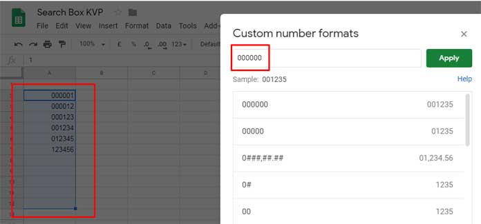
Steps to add leading zeros using number format in Google Sheets

Leading zeros will be added to the selected range. It keeps the number format. You can check that by summing the numbers in the cells where the above formatting applied.

How to Add a Hyphen to Separate Each Four Digits?

You may have seen credit card (CC) numbers automatically get hyphenated as you type in online forms. We can do that using number formatting as above in Google Sheets.

In the third step above, use the following custom number formatting instead of 6 zeros.

0000-0000-0000-0000

Enter the number first. Then format the cell or range as above.

The Drawback of Number Formatting

There is a drawback to this method. Since we are using number format, the formatting will be applied to the numbers entered only. You can’t add leading 0s to text strings or alphanumeric characters as above.

In that case, format the range to text and manually enter the zeros as mentioned at the beginning or follow the below formula approach.

Pad Zeros to Existing Text Using Rept, Len and Ampersand

Assume you have already the text strings or numbers in a column. You want to add 0s in front of them.

Let’s see how can we do that using the REPT, LEN, and Ampersand (&) combination formula in Google Sheets.

First, decide the total length of the string or number of digits. I am considering the length of the string as 10 or 10 digits.

The range to pad 0s to numbers/text string/alphanumeric characters is A2:A11.

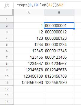
Pad zeros to existing text in Google Sheets

Enter this formula in cell B2 and copy it down.

=rept(0,10-len(A2))&A2

Alternatively, we can rewrite the above formula as an array formula to pad a certain number of zeros in front of existing text strings or numbers. In cell B2 key this array formula in.

=ArrayFormula(rept(0,10-len(A2:A11))&A2:A11)

If you happen to see the #REF! error, make sure you deleted any values in the range B3:B because array formulas need blank cells (array) to populate the results.

How Can We Remove the Leading Zeros in Google Sheets?

If the leading zeros in Google Sheets are added using the custom number format as above follow the below steps.

Removing Zeros Added Using Custom Number Format (By Undo Formatting)

Select the range/array containing the numbers formatted. Then go to Format > Number and select “Automatic”. This will clear the formatting (leading zeros) from the selected range.

What about removing leading zeros in a text formatted range?

Removing Zeros Added Using Text Format (By Using Regex)

In the beginning, I have explained two text formatting methods to get leading zeros. It doesn’t matter which method you adopt to get leading zeros. You can’t unformat it.

The only solution is using a formula in another column to remove the leading zeros. I am using the popular REGEXEXTRACT text function here.

The Regex Formula for the Range A2:A:

=ArrayFormula(REGEXEXTRACT("0"&A2:A,"0+(.*)"))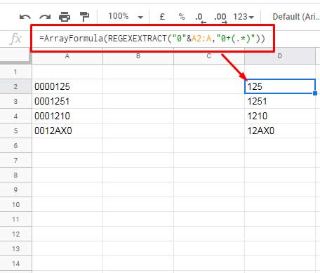

Removing leading zeros in Google Sheets using Regex

Want the above Regex for a single cell for example cell A2?

Then remove the ArrayFormula function (including open/close brackets) and change the reference A2:A to A2 in the formula above.

If there are no alphanumeric characters in the range and contain only text formatted numbers, you can use the below formula instead of using the Regex.

=ArrayFormula(A2:A5*1)