The ISNONTEXT function checks whether a value is anything other than text and returns TRUE or FALSE based on the result. It is the opposite of the ISTEXT function.
It returns TRUE for numbers, dates, times, timestamps, empty cells, and Boolean values. In contrast, the ISTEXT function returns FALSE for these cases and TRUE only for text values.
Below, you’ll learn how to use the ISNONTEXT function in Google Sheets. Additionally, you’ll see how it differs from the ISNUMBER function in a side-by-side comparison.
ISNONTEXT Function: Syntax and Formula Examples
Syntax:
ISNONTEXT(value)Where value is the value to be checked.
Example:
Assume the value in cell A1 is "Prashanth". Since it is text, the formula will return FALSE.
=ISNONTEXT(A1)The function will return TRUE if cell A1 is empty, contains a number, date, time, timestamp, TRUE, or FALSE.
Real-Life Example
Let’s see how to use the ISNONTEXT function in an IF logical test.
Example Dataset:
The dataset contains sales data, including the date, item description, delivery area/location, quantity, and unit rate in columns A to E. Column F is left blank, and in this column, you want to calculate the price for each item by multiplying the quantity by the unit rate.
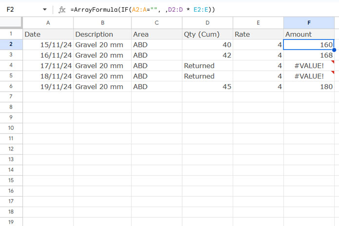
You can use the following formula in cell F2, which will automatically expand the result:
=ArrayFormula(IF(A2:A="", ,D2:D * E2:E))However, if there are any text values in columns D or E, the formula will return #VALUE!.
To handle these errors, you can wrap the formula in the IFERROR function:
=ArrayFormula(IFERROR(IF(A2:A="", ,D2:D * E2:E)))To keep the calculation going without errors, you can use the ISNONTEXT function. Here’s the updated formula:
=ArrayFormula(IF(A2:A="", ,IF(ISNONTEXT(D2:D), D2:D * E2:E, D2:D)))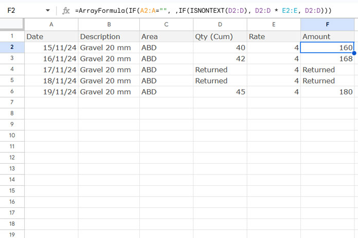
This formula will perform the multiplication only when the values in column D are not text. If the value in column D is text, it will simply return the value from column D.
ISNONTEXT vs ISNUMBER: Output Comparison
Below is a comparison of the outputs returned by ISNONTEXT and ISNUMBER for different values:
| Value | ISNONTEXT | ISNUMBER |
| 20 | TRUE | TRUE |
| 03/12/2024 | TRUE | TRUE |
| 10:10 | TRUE | TRUE |
| 03/12/2024 10:40:20 | TRUE | TRUE |
| TRUE | TRUE | FALSE |
| FALSE | TRUE | FALSE |
| TRUE | FALSE | |
| Apple | FALSE | FALSE |
- The ISNUMBER function returns
TRUEfor numbers, dates, times, and timestamps, whereas the ISNONTEXT function returnsTRUEfor those values, plus it also returnsTRUEfor empty cells and Boolean values (TRUEorFALSE).
That’s the key difference between the two functions.


