You may want to highlight weekends in a calendar, in a column in a table, or in the taskbar area of a Gantt chart in Google Sheets. How do you do that?

Different techniques are needed for each scenario. It’s easy if you want to highlight in a column or row. However, in a timescale or calendar, you may want to match weekends and highlight the entire column.

Before we delve into examples that illustrate these different scenarios and how to handle them, please take a moment to look at the table below. It contains numbers representing days of the week.

We may need to use these numbers in my formula to highlight specific weekends.

Highlight Weekends in a Column

In the following example, I have sales dates in column A and sales quantities in column B where A1 and B1 contain the field labels.

We need to highlight A2:A for weekends Saturday and Sunday.

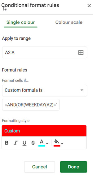
Highlight Rule:

=AND(OR(WEEKDAY(A2)=1, WEEKDAY(A2)=7), ISDATE(A2))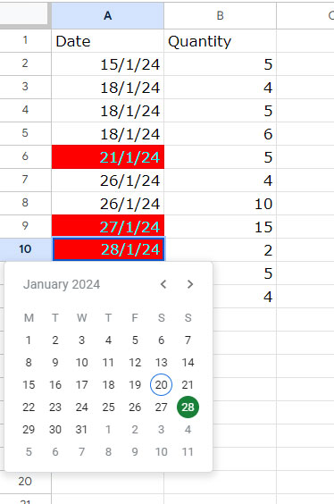

How to apply this rule in the range A2:A?

• Click on Format > Conditional formatting
• Enter A2:A under “Apply to range.”
• Under “Format rules,” select “Custom formula is,” and enter the above formula in the field below that.
• Under the “Formatting style,” pick/apply your choice and click “Done.”

Follow-Up Questions:

1. What changes should I make to highlight specific weekends such as Friday and Saturday in columns?

In the formula, replace =1 with =6 (representing Friday, you can refer to the table above).

=AND(OR(WEEKDAY(A2)=6, WEEKDAY(A2)=7), ISDATE(A2))

2. If you want to highlight only a single weekend day such as Sunday only?

You do not need the OR logical test and also require only one WEEKDAY test.

=AND(WEEKDAY(A2)=1), ISDATE(A2))

3. How to highlight the entire rows matching weekends in Google Sheets?

There are two changes required.

• In the “Apply to range,” replace A2:A with the range you want to highlight, for example, A2:B.
• In the formula, place a dollar sign in front of the column letter in cell references. So A2 will become $A2. Please see the below formula which highlights Saturday and Sunday weekends, but the entire row in the selected range.

=AND(OR(WEEKDAY($A2)=1, WEEKDAY($A2)=7), ISDATE($A2))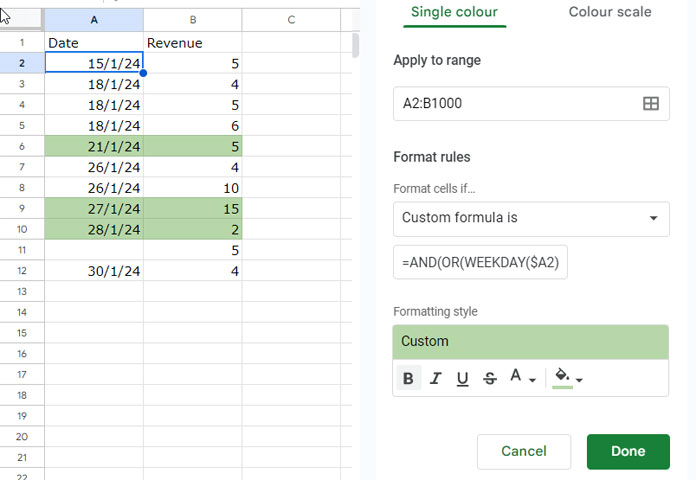

To learn the formula, you may check out: “Combined Use of IF, AND, and OR Logical Functions in Google Sheets.”

Highlight Weekends in a Calendar

You can find plenty of Google Sheets calendar templates online, and we have our own too.

Yearly Calendar

Highlighting weekends in a calendar is challenging, as each calendar may have its own formula approaches and layout settings.

Our formula (conditional format rule) will work if the days within the calendar are actual dates. You can use the ISDATE function to test whether a cell value is a date.

Another criterion is a month name in any cell in the sheet. If your template satisfies this, you can use the same formula as above, with one addition.

Example:

=AND(OR(WEEKDAY(C4)=1, WEEKDAY(C4)=7), ISDATE(C4), MONTH(C4)=MONTH($H$1&1))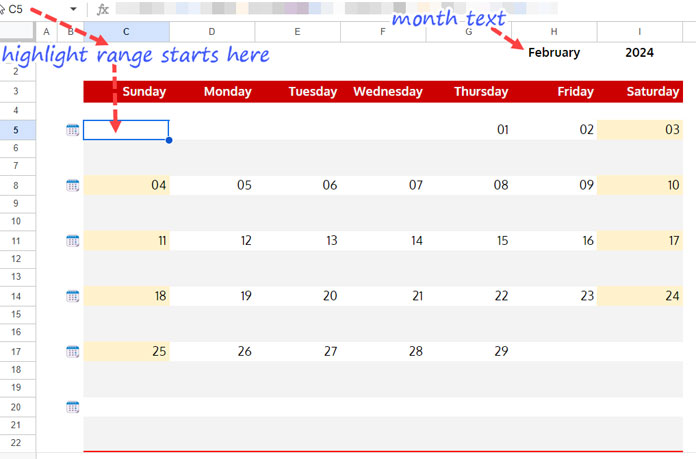

In the above example, the “Apply to range” (highlight range) is C4:I22. So, in the formula, you should use cell C4 as a reference.

The other change in the formula is the use of MONTH(C4)=MONTH($H$1&1)

It checks whether the month number of the dates in the calendar matches the month number in cell H1 (MONTH($H$1&1) converts the month text in cell H1 to the month number).

Related: Formula to Convert Month Name in Text to Month Number in Google Sheets.

Why is this necessary?

Most calendars may have dates from the previous month in the first row (week), which are hidden, and dates from the next month in the last row (week), which are also hidden.

We don’t want the formula to highlight those cells.

Notes:

A calendar may already have several formatting. You may need to drag and drop the rules according to your priority. To do that, hover your mouse pointer over the rule in question, and click on the vertical dots on the left, and drag.

To highlight specific weekends in a Google Sheets calendar, please scroll up and see the instructions under the “Follow-up questions.”

Highlight Weekends in a Gantt Chart Timescale

To highlight weekends in the taskbar area of a Gantt chart, you may need to match weekends in the timescale.

Here also, the conditional format rule will work if the values in the timescale are dates. You may check that using the ISDATE function.

Gantt Chart

Example:

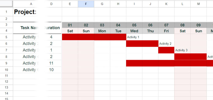
In this example, I’ve used the following formula to highlight weekends in the taskbar area. The “Apply to range” is E4:Z20.

=AND(OR(WEEKDAY(E$3)=1, WEEKDAY(E$3)=7), ISDATE(E$3))

Note: To highlight specific weekends in a Gantt chart, please scroll up and see the instructions under the “Follow-up questions.”

Resources

With the above examples, I hope you can learn to highlight weekends in specific cells, entire columns, and rows in Google Sheets. Here are some related resources to further deepen your conditional formatting expertise.

1. Highlighting Today and N Cells Below in Google Sheets Calendar
2. How to Highlight Next N Working Days in Google Sheets
3. Highlight Earliest Events Based on Date Column in Google Sheets
4. Date-Related Conditional Formatting Rules in Google Sheets
5. How to Highlight Cells Based on Expiry Date in Google Sheets
6. How to Highlight Recurring Events or Payment Dates in Google Sheets