In a table, the first row usually contains the field labels or column names. We call it headers or a header row.

Sometimes, as part of our data processing, we may require to find the header of the last non-blank cell in a row.

In short, we may require to find the last non-blank cell in the second row and return its header from the first row.

In Google Sheets, you may not find any built-in command to achieve the same. Then what’s the solution to this?

Earlier I have posted the solution to find the last non-empty column in a row. We are just required to offset that column number in the header row.

What about finding the headers of the last non-blank cells in each row?

If you want to find the column names of the last non-blank cells in each row in Google Sheets, you may copy-paste the formula in each row.

Further, we can write a different solution that expands for rows in the entire table to avoid that hassle.

In this tutorial, you will get the array and non-array solutions to return the headers/field labels of the last non-blank cells in each row.

I am starting with the sample data and a non-array solution.

Formula to Get the Header of the Last Non-blank Cell in a Row in Google Sheets

Sample Data:-

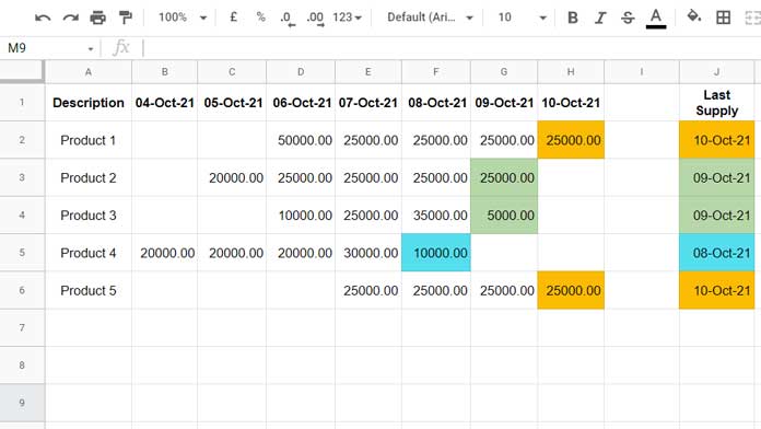
In a Google Spreadsheet, I have recorded the shipment of a few products from 04-Oct-2021 to 10-Oct-2021.

There are a total of five products.

I want to find the last shipment date of each product in cell range J2:J6.

Non-Array Solution:-

=index($B$1:$H$1,IFNA(match(2,1/(B2:H2<>""))))

Insert the above Index-Match combo in cell J2.

It will return the header of the last non-blank cell in the row range B2:H2, i.e., related to “Product 1.”

To get the last shipment date of other products, you should copy-paste the formula down.

How does this formula able to return the Header of the Last Non-blank Cell in a Row?

It’s just simple!

The Match part returns the column number (relative position) of the last non-blank cell in the range B2:H2.

You May Like: Alternatives to the XMATCH Function in Google Sheets.

As per the above example, it’s 7.

The Index offsets seven cells to the right in cell range B1:H1 and returns the field label 10-Oct-21.

When you drag the formula down, the relative row reference changes in Match, but the Index offsets in the same header row as the reference within it is absolute.

Array Formula to Get the Headers of the Last Non-blank Cells in Each Row

If you have several products or data in several rows, I recommend using an array formula for the above purpose.

It may make editing the Sheet easier in the future.

Sample Data:- Same as above.

Array Formula Solution to Get the Headers of the Last Non-blank Cells in Each Row:-

=index(
     sortn(
        sort(
           {query(split(flatten(ROW(B2:H6)&"|"&B1:H1&"|"&B2:H6),"|"),
            "Select * where Col3 is not null"),sequence(counta(B2:H6))},
           4,0
        ),
        9^9,2,1,1
     ),
     0,2
)

Insert this array formula in cell J2. If it returns #REF!, you should empty J3:J6.

You can learn this formula step by step below.

Formula Explanation

There are three main steps involved in this array formula that finds the headers/field labels of the last non-blank cells in each row in Google Sheets.

1. UNPIVOT the Evaluation Range

We want to find the last non-blanks in each row in the range B2:H6, and its header is in B1:H1.

We should unpivot this range (B1:H6) using concatenate (ampersand sign), Flatten, and Split.

What we will do here is;

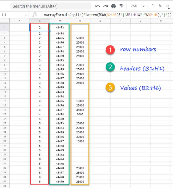
A) Combine field labels in the B1:H1 range with the values in B2:H6. We will insert a pipe delimiter in between to split them later.

In addition to that, we will add row numbers in the range B2:H6 with these values.

B) Flatten it.

C) Split it.

split(flatten(ROW(B2:H6)&"|"&B1:H1&"|"&B2:H6),"|")

D) Query it.

The second column contains dates formatted as date values. You can ignore the formatting right now.

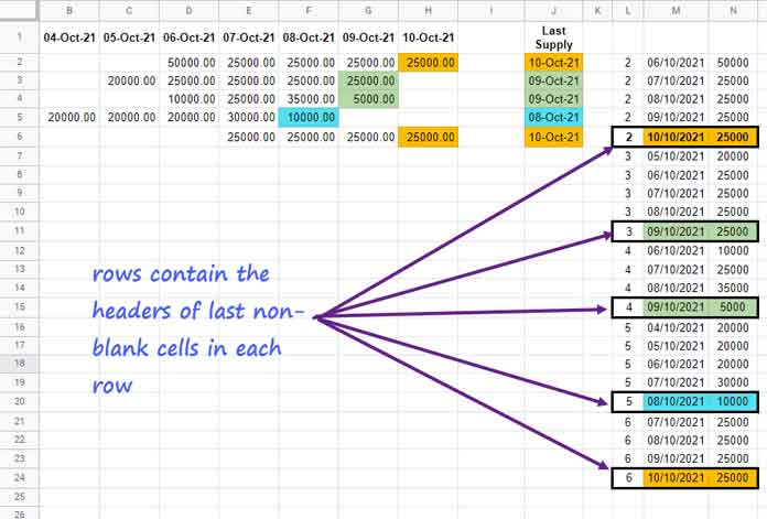
Using Query, we will remove rows that are blanks in column 3.

query(split(flatten(ROW(B2:H6)&"|"&B1:H1&"|"&B2:H6),"|"),"Select * where Col3 is not null")

Note:- Enter the above two formulas using Ctrl+Shift+Enter.

We have unpivoted the data.

Select the second column and apply Format > Number > Date.

From this column-wise (unpivoted) data, it’s easy to get the headers of the last non-blank cells in each row.

How?

Just retrieve the second column values (dates) from the last row of each row group. Here is how.

2. Flip Data Using Sorting

A) We should first generate a sequence column for the above-unpivoted data.

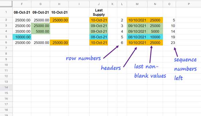
sequence(counta(B2:H6))

It will return the numbers 1 to 23 as there are 23 rows in the unpivoted output above.

B) Combine Sequence with the Unpivoted Data.

{query(split(flatten(ROW(B2:H6)&"|"&B1:H1&"|"&B2:H6),"|"),"Select * where Col3 is not null"),sequence(counta(B2:H6))}

Note:- Use Ctrl+Shift+Enter to make it work.

It will add the sequence numbers as the fourth column.

C) Flip Data Using Sorting Sequence (fourth column) in Descending Order.

sort({query(split(flatten(ROW(B2:H6)&"|"&B1:H1&"|"&B2:H6),"|"),"Select * where Col3 is not null"),sequence(counta(B2:H6))},4,0)

3. Delete Duplicates and Index to Offset

To delete duplicates based on the row numbers, we can use SORTN as below.

sortn(sort({query(split(flatten(ROW(B2:H6)&"|"&B1:H1&"|"&B2:H6),"|"),"Select * where Col3 is not null"),sequence(counta(B2:H6))},4,0),9^9,2,1,1)

We just need to get the second column from the above table. We have used Index for that.

When you use the array formula, you must ensure there are no blank rows in the range.

This way, we can Get the Headers of the Last Non-blank Cells in each Row in Google Sheets.

Related Resources

• Get the Headers of First Non-blank Cell in Each Row in Google Sheets – Array Formula.
• Google Sheets: How to Return First Non-blank Value in a Row or Column.
• How to Find the Last Value in Each Row in Google Sheets.
• Vlookup to Get the Last Non-blank Value in a Row in Google Sheets.
• Count From First Non-Blank Cell to Last Non-Blank Cell in a Row in Google Sheets.