To find the average of the smallest n values in Google Sheets, you should first know how to pick the corresponding numbers from a range.

In Google Sheets, we can use the functions such as SORTN or SMALL, for that.

Then the question is how to exclude zero values. There are options for that also, and they are QUERY and FILTER. I prefer the latter.

So in this post, you will get four formulas: Two options each for finding the average of the smallest n that includes zero and excludes zero.

1. SMALL (includes 0)
2. SORTN (includes 0)
3. SMALL + FILTER (excludes 0)
4. SORTN + FILTER (excludes 0)

What’s more, we can convert all of them into array formulas with the help of Lambdas.

How does the array formula useful?

For example, assume you have marks of students from different grades in a Spreadsheet: Ist grade in the first row, IInd grade in the second row, IIIrd grade in the third row, and so on.

Instead of writing formulas for every row, you can use an array formula that spills down from row # 1.

Average of Smallest N Values Including Zero in Google Sheets

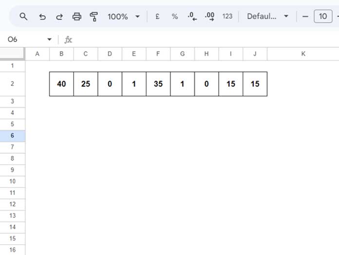
I’ve arranged the data horizontally for the test.

If your data is in a different order, I mean, in a column, you may require to make one change in the formula. I’ll point out that when the scenario comes. Here the sample data is in B2:J2.

Let’s find the average of the smallest n values in this range, and the n here is 5.

We can use either of the below two formulas to get the smallest 5 numbers, which includes 0 (zero) in Google Sheets.

SMALL Based:

=ArrayFormula(iferror(small(B2:J2,sequence(5))))

The SMALL returns the smallest 5 numbers with the help of SEQUENCE, which returns sequence numbers 1 to 5.

Do you know the role of the IFERROR?

It will remove errors when N is larger than the count of numbers in the range.

For example, we have 9 numbers in B2:J2. If n is 10, the formula will return one error value. That may cause an error in the AVERAGE calculation.

SORTN Based:

=sortn(transpose(B2:J2),5)

We have seen the core purpose of the SORTN in duplicate removal.

It returns sorted n rows and can include or exclude duplicate rows based on specified tie modes. Here we use it for returning sorted n rows.

Note:- The TRANSPOSE is not required if your data is in a column.

Wrap the above two formulas with the AVERAGE function to get the average of the smallest n numbers, including zero, in Google Sheets. Here are them.

Formula # 1 (Includes Zero):

=ArrayFormula(average(small(B2:J2,sequence(5))))

Formula # 2 (Includes Zero):

=average(sortn(transpose(B2:J2),5))

Average of Smallest N Non-Zero Values in Google Sheets

There are two functions capable of filtering a range: QUERY and FILTER. Use either of them to filter out zeros from the range.

That means, to average the smallest n non-zero values replace B2:J2 in the above formulas with the following FILTER.

filter(B2:J2,B2:J2>0)

Here are the two solutions (SMALL and SORTN) based on it.

Formula # 1 (Excludes Zero):

=ArrayFormula(average(small(filter(B2:J2,B2:J2>0),sequence(5))))

Formula # 2 (Exludes Zero):

=average(sortn(transpose(filter(B2:J2,B2:J2>0)),5))

Spill Down (Array Formula) Solutions: Including and Excluding Zero

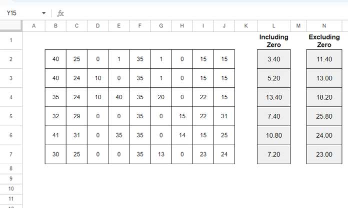
Sample Data:

How do we find the average of the smallest n values in B2:J2, B3:L3, B4:L4, and so on separately?

There are two options in front of us: Use one of our earlier non-array formulas in L2 and copy-paste it down, or use a new spill-down formula.

We have four formulas above. Out of which, we will convert two of them into array formulas.

I will pick the SORTN-based formulas, which seem best to me compared to SMALL-based ones.

In cell L2, insert the following formula to find the average of the smallest n (five here) values, including zero, in every row.

=byrow(B2:J7,lambda(r,average(sortn(transpose(r),5))))

This one excludes zeros and spills down from N2 (please see the screenshot above).

=byrow(B2:J7,lambda(r,average(sortn(transpose(filter(r,r>0)),5))))

You can use BYROW or MAP functions in Google Sheets to spill down results as above. Both are Lambda helper functions.

Since I’ve explained them in relevant tutorials, I’m skipping that here.

Any doubt, please post in the comments.