


Choose between two methods to remove duplicate values within each row in Google Sheets, each yielding distinct outputs. The choice depends on whether you want to preserve the original value positions or not.
Approach 1: UNIQUE and BYROW
This method employs the UNIQUE function along with the BYROW lambda function to eliminate duplicate values within each row and adjust their positions accordingly.
Approach 2: COUNTIFS and BYROW
In the second approach, duplicate values within each row are eliminated. It preserves the original positions of the remaining values by leaving empty cells in the place of duplicates.
Things to Consider
We use formulas for removing horizontal deduplication of value, resulting in real-time reflections of changes in the source data. Editing the result may break the formula.
If your data is final and no longer subject to editing, you can copy-paste the result as values after applying the formula, allowing for further edits.
To copy formula results as values:
- Select the cells with the formula results.
- Copy them using Ctrl + C (Windows) or Command + C (Mac).
- Right-click on the destination cells, choose “Paste special,” and select “Paste values only” or use Ctrl + Shift + V (Windows) or Command + Shift + V (Mac).
Related: Google Sheets Keyboard Shortcuts for All Popular Browsers
For simplicity and to avoid accidentally deleting the formula, put your data in one sheet and the formula in another. In our examples, both are in one sheet, but the formula can be used in a different sheet.
Finally, the solution employs a lambda-based approach for removing duplicate values within each row. Note that lambdas, known for their performance, may encounter issues or slow down your sheet with extensive data.
Remove Duplicate Values Within Each Row: UNIQUE and BYROW Solution
Let’s assume you’ve entered the date in cell A2 and listed the names of customers you interacted with on that day in B2, C2, D2, and so forth. If you’ve contacted a customer multiple times a day, you may only want to retain their first appearance. These entries extend throughout the entire month on your sheet.
How can you horizontally remove duplicate values in Google Sheets, row by row?
For the example, we are using the range A2:F5 in ‘Sheet1’, but you can apply it to a smaller or larger data range.
Formula:
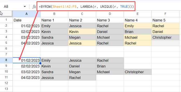
=BYROW(Sheet1!A2:F5, LAMBDA(r, UNIQUE(r, TRUE)))This formula in cell A8 (as per screenshot above) removes duplicate names horizontally, row by row, within the source data range Sheet1!A2:F5. You can use it in the same sheet or another sheet within the same workbook.
The formula produces the table after eliminating duplicate values within each row.
Formula Explanation:
The combination of BYROW and UNIQUE, as mentioned above, is equivalent to applying the following formula in cell A8 and dragging it down:
=UNIQUE(Sheet1!A2:F2, TRUE)When dragging down the formula, the ranges become Sheet1!A3:F3, Sheet1!A4:F4, and Sheet1!A5:F5, effectively removing duplicates horizontally, row by row.
By using TRUE as the second argument to UNIQUE, we ensure the removal of duplicates appearing multiple times within the same row.
Related: How to Use UNIQUE Function in Horizontal Data Range in Google Sheets
Instead of dragging the formula that uses the range Sheet1!A2:F2 down, we specify the array, i.e., Sheet1!A2:F5, within the LAMBDA to perform an array operation.
The BYROW function iterates over each row in the array Sheet1!A2:F5 and applies an unknown lambda function. The lambda function takes one argument, represented by the name ‘r’, which signifies the current element in the array.
The UNIQUE function eliminates duplicate values in ‘r’ by column.
This operation results in the removal of duplicate values in each row. Please note that this process may shift columns depending on the specific data and duplicate patterns within each row.
Remove Duplicate Values Within Each Row: COUNTIFS and BYROW Solution
When utilizing UNIQUE to remove duplicate values within each row, it’s crucial to recognize that the order of the remaining values may change. This is because UNIQUE removes duplicates without preserving the original order of values.
To retain the existing values in the same cell without shifting them to the left, leaving an empty cell where the duplicate value was present, you can implement the following COUNTIFS approach:
=BYROW(Sheet1!A2:F5, LAMBDA(r, ArrayFormula(IF(COUNTIFS(r, r, COLUMN(r), "<="&COLUMN(r))=1, r,))))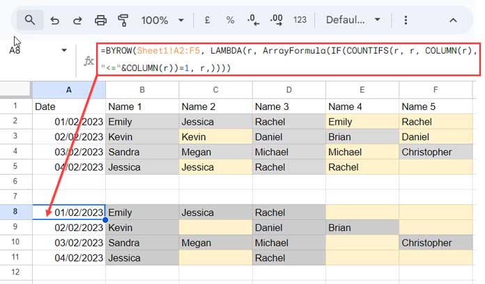
Note: The formula may display numeric values in the result for date, timestamps, or time columns. In our case, where the first column contains dates, it is recommended to select the initial column in the result table and apply Format > Number > Date for proper formatting.
Formula Explanation:
The combination of BYROW and COUNTIFS, as mentioned above, is equivalent to applying the following formula in cell A8 and dragging it down:
=ArrayFormula(IF(COUNTIFS(A2:F2, A2:F2, COLUMN(A2:F2), "<="&COLUMN(A2:F2))=1, A2:F2,))As the formula is dragged down, the ranges adapt to Sheet1!A3:F3, Sheet1!A4:F4, and Sheet1!A5:F5. This process effectively eliminates duplicates horizontally, row by row, while retaining the original positions of the remaining values.
Syntax:
COUNTIFS(criteria_range1, criterion1, [criteria_range2, …], [criterion2, …])ArrayFormula Function:
ArrayFormula(…)The ArrayFormula function is utilized due to the application of a multiple-criteria COUNTIFS function. Additionally, the COLUMN function within COUNTIFS relies on an array reference.
COUNTIFS Function:
=ArrayFormula(COUNTIFS(A2:F2, A2:F2, COLUMN(A2:F2), "<="&COLUMN(A2:F2)))This functions as a running count array formula. For example, given the values in A2:F2:
| 01/02/2023 | Emily | Jessica | Rachel | Emily | Rachel |
The formula returns {1, 1, 1, 1, 2, 2} because the last occurrences of “Emily” and “Rachel” are counted as 2.
IF Function:
=ArrayFormula(IF(COUNTIFS(…) = 1, A2:F2, ""))The IF function evaluates the result and returns the value in A2:F2 if the running count is 1; otherwise, it returns a blank cell.
BYROW Function:
=BYROW(Sheet1!A2:F5, LAMBDA(r, …))BYROW iterates over each row in the specified range (Sheet1!A2:F5), and LAMBDA defines an anonymous function that takes a row (r) as an argument.
The function within the lambda expression is the aforementioned COUNTIFS array formula, where we substitute A2:F2 with ‘r’ (the current row).
The entire formula is a concise and efficient way to deduplicate values within each row of the specified range.
Resources
Upon searching this blog, you will find over 40 tutorials covering various aspects of handling duplicate values in Google Sheets. In this tutorial, we specifically covered the removal of duplicate values within each row.
Here are ten handpicked tutorials that you may find interesting.
- Master Joins in Google Sheets (Left, Right, Inner, & Full) – Duplicate IDs Solved
- How to Exclude Duplicates in Vlookup Array Result in Google Sheets
- How Not to Allow Duplicates in Google Sheets (Data Validation)
- Assign the Same Sequential Numbers to Duplicates in a List in Google Sheets
- Make Duplicates to Unique by Assigning Extra Characters in Google Sheets
- How to Duplicate Rows Based on Start and End Dates in Google Sheets
- Find and Remove Duplicates in Google Sheets: Different Options
- Flexible Array Formula to Rank Without Duplicates in Google Sheets
- Compare Two Tables and Remove Duplicates in Google Sheets
- Removing Duplicates by Key Column in Google Sheets