


Can I use the Sumproduct function with merged cells in Google Sheets?
Yes! We can do that similar to Sumif in Merged Cells. We can virtually unmerge and fill all of the arrays in use in Sumproduct to get the correct result.
I will walk you through how to do it in Google Sheets.
What Do We Want to Achieve?
We can use Sumproduct to get the sum of products at one go. While doing so, we can include criteria to skip some rows.
In a dataset that contains multiple products such as “ISMC 75”, “ISA 75X75X6”, and “ISMB 200” (some country-specific structural steel items), we can get the sum of the product of any of the above items or all of them.
If we want to stick with any specific items, we must use criteria within the formula.
We will follow that within our example below.
Now let’s see what do we want to achieve here.
In the following example, some of the cells in the columns that contain items, unit, and unit weights are merged.
In cell F2, I have a Sumproduct formula that does the job (return the sum of the product) wonderfully.
As I have already mentioned above, some cells are merged in the array in use in the evaluation.
Irrespective of that, the Sumproudct formula in cell F2 returns the product sum as per the criteria in cell E2.
For example, when I select ISMB 200 (a structural steel item) from the drop-down in cell E2, it calculates as follows.
=2*24.2+2.5*24.2Before revealing the formula in cell F2, you should know what formula you should use when you have no merged cells in the cell range/arrays.
That is very important to know before learning how to use Sumproduct with merged cells in Google Sheets.
Sumproduct with Merged Cells In Google Sheets (Formula and Explanation)
Assume we have unmerged the data and formatted it as below.
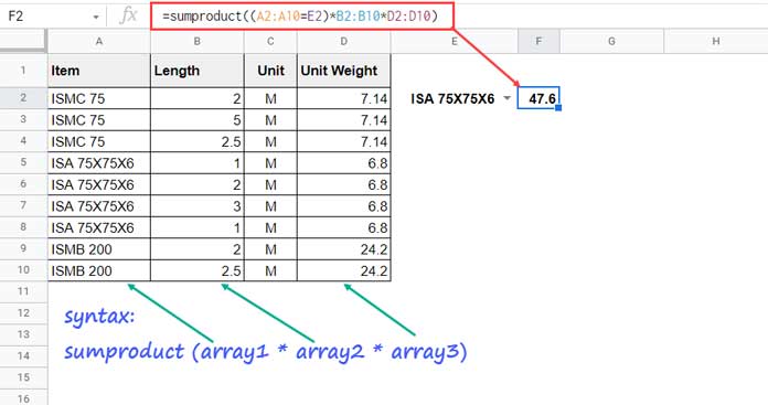
Then, we can use the below Sumproduct formula to get the sum of the product of the item selected in cell E2.
=sumproduct(
     (A2:A10=E2)*
     B2:B10*
     D2:D10
)
If you analyze this formula, you can understand that we should deal with arrays 1 (cell range A2:A10) and 3 (cell range D2:D10). Please see both of the screenshots above.
We have to unmerge them virtually and fill in data.
I mean, we should replace A2:A10 and D2:D10 with virtual LOOKUP arrays, and here are them.
A2:A10:
lookup(row(A2:A10),if(len(A2:A10),row(A2:A10)),A2:A10)D2:D10:
lookup(row(A2:A10),if(len(D2:D10),row(A2:A10)),D2:D10)Here is how to use the Sumproduct function with merged cells in Google Sheets. I have included the above two Lookup virtual arrays in it.
The formula in F2:
=sumproduct(
     (lookup(row(A2:A10),if(len(A2:A10),row(A2:A10)),A2:A10)=E2)*
     B2:B10*
     lookup(row(A2:A10),if(len(D2:D10),row(A2:A10)),D2:D10)
)
To learn the above Lookup formulas, please read my detailed tutorial here – How to Fill Merged Cells Down or to the Right in Google Sheets.
Conclusion
When you want to include more columns, you can change the following cell range references/expressions in the above lookup formula.
Replace all the cell references that are not enclosed within the ROW function with the corresponding cell range.
That’s all about how to use the Sumproduct function with merged cells in Google Sheets.
You can find below a sample sheet and additional resources to deal with merged cells.
Resources:
- Copy-Paste Merged Cells Without Blank Rows/Spaces in Google Sheets.
- How to Find the Cell Addresses of the Merged Cells in Google Sheets.
- Sort Vertically Merged Cells in Google Sheets (Workaround).
- Merge and Unmerge Cells and Preserve Values in Google Sheets.
- Sequence Numbering in Merged Cells In Google Sheets.