


Calendar week formula in Google Sheets – What’s that?
The Weeknum (see my functions guide) is the ‘only’ function to identify calendar weeks. But it returns week numbers, not week range.
What I want is the week start date to end date like 04-Feb-2019 to 10-Feb-2019 (Monday-Sunday) instead of week number 6.
Here comes the importance of my calendar week formula in Google Sheets.
Note: I have used type 2 week number calculation in which day of the week begins on Monday and ends on Sunday.
If I have used type 1, then the calendar week range will be 03-Feb-2019 to 09-Feb-2019 (Sunday-Saturday).
I will give you more info about this in the concerned formula part below. Here I am going to use the function Weekday, not Weeknum.
My calendar week formula in Google Sheets would return the week start dates and end dates in a combined form from a list of dates. Further, the formula has the compatibility to use in a date range in that the dates span different years.
See the output that returned by my calendar week formula first, then I will tell you where we can use it.
You can easily find calendar week start date and end date of any date using a simple formula. I have already explained that here – Formula to Find Week Start Date and End Date in Google Sheets.
That I am going to use in an array form to achieve our result. Actually, I have two different types of formula options. Both I will explain and provide you. You can pick the suitable one for you.
The Purpose of Calendar Week Formula in Google Sheets
The purpose of using my calendar week formula is simple that is to combine the start date of a week with the end date. But the real purpose is different. With that formula we can create weekly summary reports like;
- The weekly average of sales during the period 01/01/2018 to 16-02-2019 (daily data to weekly average).
- The weekly sum of sales that spanned several years (daily data to weekly sum).
And finally;
- The weekly count of receipt of goods (number of truck loads) for a given period (daily data to weekly count)
If you are happy to get the summary based on the week numbers, then the things will be easy for you.
We can use Query for this and you can see one example in my earlier tutorial here – How to Create A Weekly Summary Report in Google Sheets.
You can summarise a date range based on the calendar week, not week number but week start and end dates as the column heading, using my calendar week formula in Google Sheets.
In this tutorial, I am not going into the summarisation part. Here you can learn how to get calendar week start date and end dates as the column heading.
The calendar week wise summary, that you can learn in one of my upcoming tutorial which is already in the pipeline. I will definitely provide you the link. I mean I will update this post with that link included.
Combine Week Start and End Dates Using Calendar Week Formula
Sample Data:
I have some random dates in column A like;
The rows A2
I want to show you the multi-year compatibility of my formula. That’s why I have included dates that span two years.
Also, even if the dates are unsorted, it won’t affect my formulas. So you are safe with dates in any sort order – ascending, descending or random order.
There are two types of formulas I have to offer. Let’s begin with the formula 1. This is a combination formula so I will take you to it step by step.
Step 1:
How to Return Week Start Dates of a Given Daily Date Range
Formula # 1 (temporarily apply in cell B2)
=ArrayFormula(A2:A58-WEEKDAY(A2:A58,2)+1)This formula will place the week start dates in B2
Wrap the above formula with the Unique function to remove the duplicate week start dates.
Formula # 2 (modify the formula in cell B2)
=unique(ArrayFormula(A2:A58-WEEKDAY(A2:A58,2)+1))Now we must sort this formula output. Just wrap the above formula with the SORT function. You can remove the ArrayFormula when using SORT.
Formula # 3 (modified in cell B2)
=sort(unique(A2:A58-WEEKDAY(A2:A58,2)+1))Here is the output.
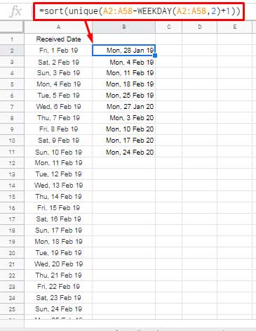
See column B2
To learn further about weekday types, please check my complete date function guide for Weekday.
Step 2:
How to Return Week End Dates of a Given Daily Date Range
Here I am not going to take you through all the above steps. The formula is the same except the +6.
Formula (temporarily apply in cell C2)
=sort(unique(A2:A58-WEEKDAY(A2:A58,2)+1+6))This formula simply adds 6 days to the week start dates to get the week end dates. Simple logic, right?
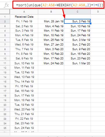
See the weekend dates are Sunday. To change that to Saturday, as I have mentioned above, change the type 2 in Weekday to 1.
The above outputs you can use in formulas like Sumif, Countifs, Averageifs to sum, count, average based on date range in Google Sheets.
Step 3:
Combine the Week Start and End Dates to Create Columns for Calendar Week
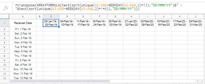
You can combine the week start dates and end dates and transpose to columns as shown in screenshot # 1 in the beginning. There see the data in the range C1:L1.
Here is the step-by-step instructions. Just try to understand the below formulas.
=ArrayFormula(B2:B11&" - "& C2:C11)This formula can combine the columns that contain week start dates (B2:B) and end dates (C2:C) then
- It will cause losing the date format.
- It uses the helper columns B and C.
I have earlier posted a Google Sheets tutorial, that well explains how to concatenate a date with text, or a
Must Check: Combine Text and Date in Google Doc Spreadsheet Using Formula.
I am going to use that method here. Then I will show you how to remove the helper columns. Take note of the use of the Text function.
=ArrayFormula(text(B2:B11,"DD/MMM/YY")&" - "&text(C2:C11,"DD/MMM/YY"))Now replace B2:B11 with the formula in B2 and C2:C11 with the formula in C2. That formula will be as follows.
=ArrayFormula(text(sort(unique(A2:A58-WEEKDAY(A2:A58,2)+1)),"DD/MMM/YY")&" - "&text(sort(unique(A2:A58-WEEKDAY(A2:A58,2)+1+6)),"DD/MMM/YY"))If I have given this formula in the beginning, definitely some of you may have left reading thinking the formula is quite complicated, right?
Finally, wrap the formula with Transpose to move it to columns. That will be the said Calendar Week Formula in Google Sheets
=transpose(ARRAYFORMULA(text(sort(unique(A2:A58-WEEKDAY(A2:A58,2)+1)),"DD/MMM/YY")&" - "&text(sort(unique(A2:A58-WEEKDAY(A2:A58,2)+1+6)),"DD/MMM/YY")))Please refer to the first screenshot for the formula output.
Option # 2
I have promised you there is one more formula with me. You can replace the formula that I have used in cell B2 (step 1) with;
=sortn(A2:A58-WEEKDAY(A2:A58)+1,9^9,2,1,true)and C2 (step 2) with;
=sortn(A2:A58-WEEKDAY(A2:A58)+1+6,9^9,2,1,true)You can combine this formula as per the instructions which are given under step 3. The SORTN in the above two formulas replaces the Unique and Sort. This’s is just for your information.
Conclusion:
You can soon expect a tutorial in that I will make use of the above calendar week formula in Google Sheets. It’s about a weekly summary based on calendar weeks.
Update: Summarize Data by Week Start and End Dates in Google Sheets.
Thanks for the stay. Enjoy!
Hello, In your first screenshot, the formula has calculated the dates perfectly.
What was the formula you have used in D1, E1, etc.?
Hi Sushil,
I have just one calendar week array formula in cell C1 that returns values in C1:L1.
That’s the third formula from bottom to top (just above subtitle Option # 2).
Can I include a “most recent” date where it would post the most recent week of an item that matches a particular value from a selected range (data validation)?
Hi, Ashley,
Please share a sample.
How can I tweak this so that it shows all weeks (even if there were 0 orders for that week)?
Thank you!
Hi, Jordon,
In my calendar week formula, replace the range A2:A58 (it appears four times, so replace all the four) with the below SEQUENCE formula.
sequence(days(max(A2:A58),min(A2:A58))+1,1,min(A2:A58))What does this Sequence do then?
It populates dates from min date in the range A2:A58 to max date in the range A2:A58. So the formula will return all the weeks irrespective of orders.