


Do you know how to use Google Sheets Query to filter numbers only from a column that contains mixed data types?
With the Filter function, it’s easy to do. But Query is capable of manipulating data, so you may consider learning it.
Quite recently, I was trying to do a percentage calculation in Query using the Count aggregation function in it. But sadly, the Count in Query counts both texts and numbers.
Further, as you may know, the Google Sheets Query function operates unpredictably when mixed data types are in a single column.
In such cases, the majority data type determines the data type of the column in the Query.
The other values, which means the minority data types, are considered null values.
At this juncture, filtering numbers only from a column in Query is relevant.
How to Use Google Sheets Query to Filter Numbers Only From Mixed Type Data in a Column
First, let us see the formula and example. Then I will tell you what may happen if we apply the count aggregation function with this formula.
We will see first how to use the formula in a single column.
Single Column Query

Formula:
=QUERY(A3:A,"select A where A matches '[0-9\-.]+' ",0)With this example, I hope you can learn how to use Google Sheets Query to filter numbers only.
Here I’ve used the Matches regular expression in the “Where” clause.
You can follow this example in your sheet and filter numbers only from the mixed data type column.
Please note that the values returned by the above formula might be in text format.
So how to convert those numbers in text format back to numeric values in Google Sheets Query? See that formula.
=ARRAYFORMULA(VALUE(QUERY(A3:A,"select A where A matches '[0-9\-.]+' ",0)))I’ve just used the Value function and ArrayFormula to convert the numbers from text format to number format.
I hope you could be able to learn how to use Google Sheets Query to filter numbers only when a column has mixed data types.
Query to Filter Numbers From Mixed Data Type Column: Real-Life Use
Now see two Query formulas below. Both of them count column A with and without filtering out text values.

The above two example formulas show how to use Query in a mixed data type column to get the desired result.
The formula with the red border counts all the values in column A.
But the answer may or may not be correct as Query sometimes skips values in such mixed data type columns.
Formula 1:
=QUERY(A3:A,"Select A,count(A) group by A label Count(A)''")But the second formula with the blue border (I’ve updated it below) filters the column for numeric values and then applies the count.
Formula 2:
=QUERY(
     ARRAYFORMULA(VALUE(QUERY(A3:A,"select A where A matches '[0-9\-.]+' ",0))),
     "Select Col1, Count(Col1) group by Col1 label Count(Col1)''"
)
Note:- Colum identifiers should be Col1, Col2, … instead of A, B,… when using an expression as data in Query.
Please check the output of both formulas on the screenshot to understand the difference.
Query in Multiple Columns and Filtering Numbers
We usually use Query with multiple-column data. You may not be able to apply the same above VALUE approach in that case.
So you should know how to use Query to filter numbers only from a mixed data type column when there is more than one column in the table.
Below I’ve two columns. I want to group column A and sum column B for only the data type in column B is number.
The following formula would return the “Unable to parse query string for Function QUERY parameter 2: AVG_SUM_ONLY_NUMERIC” error.
=query(A3:B,"Select A,sum(B) where A is not null group by A")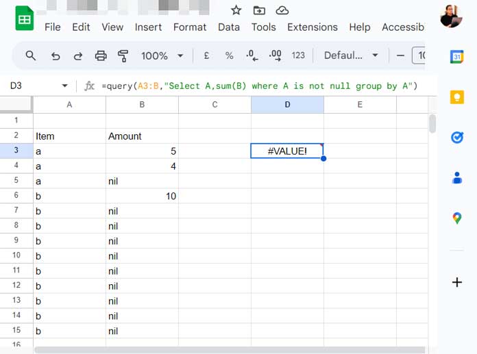
We can use the below Query to filter rows containing numbers only in the mixed data type column B.
=QUERY(A3:B,"select * where B matches '[0-9\-.]+' ",0)To perform the aggregation, we must format the values in the second column into numbers. We can take the help of HSTACK, LET, and CHOOSECOLS for that.
=LET(
     data,
     QUERY(A3:B,"select * where B matches '[0-9\-.]+' ",0),
     HSTACK(
                 CHOOSECOLS(data,1),
                 ARRAYFORMULA(VALUE(CHOOSECOLS(data,2)))
     )
)
How do I use it?
In the above formula, replace the Query formula with your Query formula.
Then specify the individual columns as comma separated within the HSTACK.
I mean, CHOOSECOLS(data,1) returns the first column, and ARRAYFORMULA(VALUE(CHOOSECOLS(data,2))) returns the second column after converting values to numbers.
If your range is A3:C and you want to extract three columns, specify CHOOSECOLS(data,3) within the HSTACK for the third column.
I’m leaving the aggregation part. You now have a cleaned data set. So you can perform other tasks on it.
That’s all for now. Enjoy!
What if we want otherwise, to show non-numeric only?
Hi, Kai,
This formula may work.
=QUERY(A3:A,"select A where A matches '[^0-9]+' ",0)