Matching multiple values in a column is a simple task in Google Sheets. But there is one key point, i.e., case sensitivity.

Usually, we follow three types of matching: Case-insensitive, case-sensitive, and partial match. We can further bifurcate the last one with case sensitivity.

Let’s consider a list of auto spare parts as the sample. The range is A2:A in one of my Google Sheets files.

I have an inquiry for three parts: Battery Box, Battery Plate, and Battery Cap.

How do I find out if all three parts are available by searching the inventory with a formula?

We should match multiple values, i.e., Battery Box, Battery Plate, and Battery Cap, in column A and get the count of matches.

If that is equal to the count of required spare parts, all parts are available with us. Please find the examples below.

Match Multiple Values in a Column: Case-Insensitive Formula

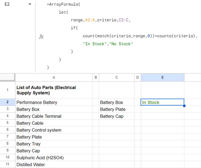
We will specify the search values, i.e., Battery Box, Battery Plate, and Battery Cap, in C2:C. The spare parts list is in A2:A.

We will use the LET function to name C2:C as the criteria and A2:A as the range. That will make the formula easy to read.

Formula # 1:

=ArrayFormula(
     let(
          range,A2:A,criteria,C2:C,
          if(
               count(match(criteria,range,0))=counta(criteria),
               "In Stock","No Stock"
          )
     )
)

If you want to specify the part names to lookup inside the formula, replace C2:C with the following VSTACK formula.

vstack("Battery Box","Battery Plate","Battery Cap")

Anatomy of Formula # 1

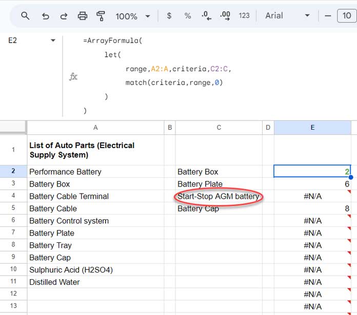
The MATCH function matches multiple values (criteria) in the range and returns relative position for matches and #N/A for mismatches.

For example, in the following test, the formula returns #N/A against the criterion “Start-Stop AGM battery” since it is not available in the range.

We have used IF in the original formula to test the MATCH result in the following syntax:

if(count(match_result)=counta(criteria),"In Stock","No Stock")

Can we use XMATCH instead of the MATCH function for multiple matches of values in a column in Google Sheets?

Yes! In the original formula, replace match(criteria,range,0) with xmatch(criteria,range).

One more thing. The role of ArrayFormula is to support matching multiple values (criteria). Without this or an equivalent array function such as INDEX, we would have limited to using C2 instead of C2:C.

Match Multiple Values in a Column: Case-Sensitive Formula

To differentiate between lower-case (small) and capital (upper) letters when matching multiple values, use the following formula in Google Sheets.

Formula # 2:

=ArrayFormula(
     let(
          range,unique(A2:A),criteria,unique(C2:C),
          if(
               sum(--regexmatch(range,"^"&textjoin("$|^",true,criteria)&"$"))=counta(criteria),
               "In Stock","No Stock"
          )
     )
)

For example, you have two different items: AQ101A and AQ101a.

Formula # 1 would treat them as the same item, but Formula # 2 would treat them as two different items.

Anatomy of Formula # 2

This formula replaces the MATCH part in Formula # 1.

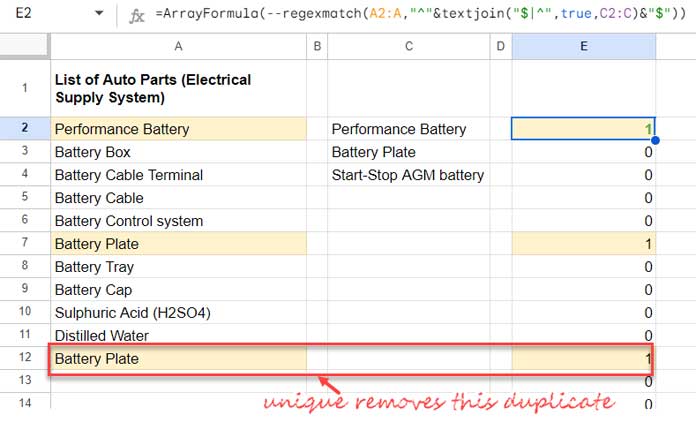
--regexmatch(range,"^"&textjoin("$|^",true,criteria)&"$")

The above REGEXMATCH formula part returns 1 for matches and 0 for mismatches.

We wrapped this formula part with SUM instead of COUNT since we have a result range of 1 and 0, unlike numbers and #N/A in MATCH, where COUNT omits the error values. Please see column E in the images below and above.

Further, we have applied UNIQUE to the range and criteria since the above formula returns match against the range, not against the criteria. So, duplicates can cause issues (please see the image below).

The IF logic is the same in Formula # 1 and Formula # 2.

The above is the case-sensitive way to match multiple values in a column in Google Sheets.

Note:- Searches in REGEXMATCH use RE2 regular expressions. So if your search string contains a metacharacter like *+?()|,, you must escape them.

For example Sulphuric Acid \(H2SO4\) searches for the item Sulphuric Acid (H2SO4).

What about the partial matching of multiple values in a column?

Partial Match Multiple Values in a Column: Case-Sensitive and Insensitive Formulas

Unlike the above two, the partial match has one issue.

You will get several matches if you partially match Battery and Sulphuric Acid in A2:A.

So matching the search result count/sum with the criteria count won’t work.

So we search for one value and aggregate that search result. Then we use BYROW Lambda to repeat the same with the second value, and so on.

For the partial match, we will use the SEARCH and FIND functions. The latter is for case-sensitive partial matches of multiple values in a column.

If we consider Formula # 2, we replaced count(match(criteria,range,0))=counta(criteria) with the below-highlighted parts for partial matches.

Formula # 3 (Case-Insensitive):

=ArrayFormula(
     let(
          range,A2:A,criteria,C2:C,
          if(
               countif(byrow(tocol(criteria,1),lambda(r,count(search(r,range)))),">0")=counta(criteria),
               "In Stock","No Stock"
          )
     )
)

Formula # 4 (Case-Sensitive):

=ArrayFormula(
     let(
          range,A2:A,criteria,C2:C,
          if(
               countif(byrow(tocol(criteria,1),lambda(r,count(find(r,range)))),">0")=counta(criteria),
               "In Stock","No Stock"
          )
     )
)

That’s all. Thanks for the stay. Enjoy!