


This post explains converting a date to a string in Google Sheets using the long-winded approach for Query criteria.
As I began drafting a tutorial on the Google Sheets Query function today, I realized the importance of covering related topics beforehand. Why? Because a thorough understanding of the Query function becomes necessary in certain scenarios.
One such scenario arises when dates appear in our data, and we intend to utilize them as a criteria column in a Query filter. It is crucial to comprehend how to employ dates as criteria in Query effectively.
While you can typically enter a date in any cell and reference it as criteria, doing so directly in Query might yield inaccurate results.
This is because, in Query, the date should be specified as a string literal in the format yyyy-mm-dd. For this conversion, we can follow either the long-winded or compact approach.
The recommended method is as follows: assume you want to use a date in cell A1 as a criterion. In cell B1, adopt the so-called long-winded or compact approach to convert this date, and then use cell B1 as your criteria.
This tutorial guides you through the process of converting a date to a text string in Google Sheets for Query use.
Should I Limit Myself to Converting Date to String Using the Long-winded Approach Only?
No! You can also convert a date using the compacted approach, and that is the recommended one. However, understanding both approaches is necessary when working on a shared Google Sheet.
If someone has used the long-winded approach, you might find it challenging to comprehend the formula in use. Therefore, it’s advisable to learn both methods and opt for the compacted one when writing a query.
Converting a Date to String Using the Long-winded Approach in Google Sheets
To convert a date to a string using the long-winded approach, you should first familiarize yourself with three date functions and a text function.
I will explain each function one by one. The following are the three simple date functions in use, followed by the text function.
Year Function in Google Sheets:
Syntax:
YEAR(date)Use this function to retrieve the year from a given date.
For example, if the date in cell A6 is 20/08/2017, applying this function will yield the result 2017.
=YEAR(A6)Day Function in Google Sheets:
Syntax:
=DAY(date)Utilize this function to obtain the day of the month from a given date. Suppose the date is 20/08/2017; using this function will produce the result 20.
=DAY(A6)Month Function in Google Sheets:
Syntax:
MONTH(date)Employ this function to extract the month from a given date. For instance, consider the date as 20/08/2017; applying this month function will result in 8.
=MONTH(A6)You have now acquired the necessary date functions to convert a date to a string in Google Sheets using the long-winded approach.
Text Function:
Syntax:
TEXT(number, format)The aforementioned date functions will yield numbers. The TEXT function will be employed to convert these numbers into text strings.
Formula and Explanation
We are converting the date to text using the long-winded method in the “YYYY-MM-DD” format, supported in the Query function.
Suppose cell A6 contains a date, for example, “20/08/2017”. The following formula will convert it to the text string “2017-08-20”:
=TEXT(YEAR(A6), "0000") & "-" & TEXT(MONTH(A6), "00") & "-" & TEXT(DAY(A6), "00")Formula Explanation:
Let’s break down the components of this formula:
TEXT(YEAR(A6), "0000"): This part extracts the year and formats it as a four-digit number using the TEXT function with the format code “0000”. This ensures that the year is displayed with leading zeros if necessary.TEXT(MONTH(A6), "00"): This part extracts the month and formats it as a two-digit number with leading zeros if necessary.TEXT(DAY(A6), "00"): This part extracts the day and formats it as a two-digit number with leading zeros if necessary.- The three results from the above steps are concatenated using the
&operator, and hyphens (“-“) are inserted between them. This results in the final string in the format “YYYY-MM-DD”.
So, if the date in cell A6 is “20/08/2017”, the formula would convert it to the string “2017-08-20”.
You have now learned how to convert a date to a string in Google Sheets using the long-winded approach. Next, we’ll explore the compact method of conversion.
Converting a Date to String in Google Sheets Using the Compact Method
It’s quite easy to convert a date to a string using the compact method in Google Sheets. First, take a look at the formula below:
=TEXT(A6, "yyyy-mm-dd")The TEXT function will convert the date in cell A6 to the “YYYY-MM-DD” format.
Query Example
Now, let’s delve into two Query formulas where we apply date conversion to filter a column.
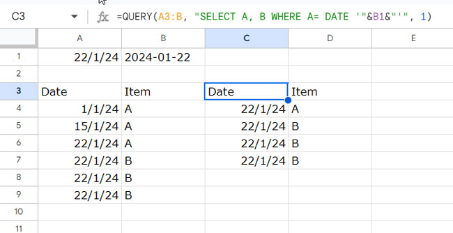
In the forthcoming examples, the data to filter is situated in cells A3:B, with column A containing dates and column B containing items.
The objective is to filter the table based on the date criterion in cell A1. However, the date in cell B1 will serve as the criterion, where I’ve utilized the compact method for date conversion.
Formula in cell B1:
=TEXT(A1, "YYYY-MM-DD")Query in cell C3:
=QUERY(A3:B, "SELECT A, B WHERE A= DATE '"&B1&"'", 1)To view the screenshot, please scroll up to the top of this page.
Instead of converting the date, you can directly use it within the Query formula. Here are two formulas, the first using the compact approach, and the second using the long-winded approach.
Compact Approach: ✅
=QUERY(A3:B, "SELECT A, B WHERE A= DATE '"&TEXT(A1, "YYYY-MM-DD")&"'", 1)Long-winded Approach:
=QUERY(A3:B, "SELECT A, B WHERE A= DATE '"&TEXT(YEAR(A6), "0000") & "-" & TEXT(MONTH(A6), "00") & "-" & TEXT(DAY(A6), "00")&"'", 1)Resources
I have explained two ways to convert a date to a string for use in Query as a criterion. Here are some additional resources that will assist you in navigating Query when your data contains a date field/column.
- How to Use Date Criteria in Query Function in Google Sheets [Date in Where Clause]
- How to Format Date, Time, and Number in Google Sheets Query
- How to Use the Datediff Function in Google Sheets Query
- How to Use DateTime in Query in Google Sheets
- Month Name as the Criterion in Date Column in Query Function in Google Sheets
- How to Use the toDate Scalar Function in Google Sheets Query
- How to Use Date Values (Date Serial Numbers) in Google Sheets Query
Thank you very much for the post! It teaches very clearly how to do it.
I’m having a little problem related to dates in Google Sheets Query.
I’m using this formula:
=QUERY(IFERROR(IFERROR(IMPORTRANGE('URL Import'!C2;'URL Import'!E2);
IFERROR(IMPORTRANGE('URL Import'!C2;'URL Import'!F2);
IFERROR(IMPORTRANGE('URL Import'!C2;'URL Import'!G2)))));"select *")
This “trick” solves an update problem that sometimes happens with the query function but when I use the
"select year(Col8)"instead of just"select *", it shows the following error:Can’t perform the function year on a column that is not a Date or a DateTime column
I hope you could help me.
Thank you!
Hi Lucas,
How many columns does your Query return? I could only see one column. If that’s the case, how do you use Col8 in your formula?
Additionally, it appears that you are incorrectly using the IFERROR function.