


Mastering the combined use of IF, AND, and OR logical functions is essential for conquering Google Sheets. This combination is one of the most commonly used formulas in Google Sheets and Excel.
In this tutorial, you will learn how to use the important logical functions IF, AND, and OR in Google Sheets, as well as how to use them in combination.
Logical functions are very easy to use if you have good examples. You can find examples of logical functions online, but there are not many resources on their combined use.
When you use logical functions in combination, it expands the usefulness of some logical functions.
I believe it is rare to find simple examples of the combined use of logical functions. Here, I will explain to you the combined use of IF, AND, and OR logical functions in Google Sheets in the simplest way possible.
Some of you may be familiar with Microsoft Excel’s logical functions. If you know IF, AND, and OR logical functions in Excel, you can use them similarly in Google Sheets. There are no changes in the syntax.
This is also true for the combined use of IF, AND, and OR logical functions. There are no changes in the use of this combination in either spreadsheet application.
It is easy to use logical functions individually, but they are more powerful when you use them in combination.
In this easy-to-follow Google Sheets tutorial, you will learn how to use logical functions in combination.
What Are Spreadsheet Logical Functions?
Logical functions are used to test values and make decisions based on those tests. We can use them in Google Sheets to automate a variety of tasks. They can be part of many complex formulas in Google Sheets.
There are four main logical functions: IF, AND, OR, and NOT. We can use them individually or combine them to create more complex logical expressions.
The most common combinations are IF, AND, and OR. NOT is less common, but you can find information on its use in another tutorial here: How to Use NOT Function in Google Sheets in Logical Test.
Logical Functions IF, AND, and OR in Google Sheets
In this section, we will learn how to use the logical functions IF, AND, and OR in Google Sheets.
Use of Logical Function IF: How to
The IF logical function is used to test whether an argument is TRUE or FALSE. If TRUE, the function returns one value, and if FALSE, it returns another value.
Syntax:
IF(logical_expression, value_if_true, value_if_false)Example: In a cell, for example, cell A1, put the value 50. Type any of the below formulas in cell B1.
Formula 1:
=IF(A1>50,"Passed", "Failed")Where:
A1>50is thelogical expression."Passed"is thevalue_if_true."Failed"is thevalue_if_false.
Formula 2:
=IF(A1>50,A1*20, A1*10)Where:
A1>50is thelogical expression.A1*20is thevalue_if_true.A1*10is thevalue_if_false.
In the first logical test, if the value in cell A1 is above 50, then the formula in cell B1 will return “Passed”, else it will return “Failed”.
In the second logical test, if the value in cell A1 is above 50 the result would be A1*20 else A1*10.
Suppose the value in A1 is 50. The second logical test formula would return 50*10 = 500.
I hope you can understand this. Still, having any doubts? Then switch to my dedicated IF function tutorial.
Use of Logical Function AND: How to
The AND function returns TRUE if all of the provided arguments are logically true; otherwise, it returns FALSE. It is a more useful tool in an IF, AND, OR combination.
Syntax:
AND(logical_expression1, [logical_expression2, ...])Example:
=AND(A1>10,A1<100)Where:
A1>10is thelogical_expression1.A1<100is thelogical_expression2.
This formula, using comparison operators, tests whether the value in cell A1 is greater than 10 and less than 100. If the value in cell A1 meets this condition, the AND formula returns TRUE; otherwise, it returns FALSE.
In the following example, the formula tests whether the values in cells A1, A2, and A3 are equal to 50.
=AND(A1=50,A2=50,A3=50)Where:
A1=50is thelogical_expression1.A2=50is thelogical_expression2.A3=50is thelogical_expression3.
It would evaluate to TRUE if all of the conditions match (tests are passed), else FALSE.
Use of Logical Function OR: How to
The OR function returns TRUE if any of the provided arguments are logically true; otherwise, it returns FALSE. It is most useful when we use it in an IF, AND, OR logical combination in spreadsheets.
Syntax:
OR(logical_expression1, [logical_expression2, ...])Example:
=OR(A1=10,B1=10)Where:
A1=10is thelogical_expression1.B1=10is thelogical_expression2.
This formula would return TRUE if any of the values in cell A1 or B1 is 10.
You can learn IF, AND, and OR logical functions easily from the following combined formula examples.
How to Use Logical Functions in a Combined Form in an Excel or Google Doc Spreadsheet
You may have noticed that I have not yet explained the real-life use of AND and OR logical functions. They simply return TRUE or FALSE. How do we use them in real life?
The following combined use of IF, AND, and, OR logical functions will clear your doubts about using these functions.
Examples of Combined Use of IF, AND, and OR Logical Functions
First, type the contents as shown in the screenshot into a spreadsheet, regardless of whether you are using an Excel spreadsheet or a Google Docs spreadsheet.
You can omit Condition 1, Condition 2, and Condition 3 (that is, keep the range E3:G3 blank) because we will apply logical functions there later.
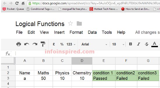
We only require values in B3, C3, and D3 for the logical tests. These are the marks of a student in three subjects in a school examination out of 50.
I hope you have typed the above data.
Now, here are the formula examples for the combined use of IF, AND, and OR logical functions in Google Sheets:
1. Condition 1 (E3):
=IF(
     OR(B3>49,C3>49,D3>49),
     "Passed",
     "Failed"
)
2. Condition 2 (F3):
=IF(
     AND(B3>49,C3>49,D3>49),
     "Passed","Failed"
)
3. Condition 3 (G3):
=IF(
     OR(AND(B3>49,C3>49),AND(B3>49,D3>49), AND(C3>49,D3>49)),
     "Passed",
     "Failed"
)
Enter the first formula under “Condition 1”, the second formula under “Condition 2”, and the final formula under “Condition 3.”
What Do These Combined Logical Functions Do?
1. The formula in cell E3 returns “Passed” if the marks scored in any subject are greater than 49 (OR logical test with IF).
OR returns TRUE if any of the provided arguments, i.e. B3>49 or C3>49 or D3>49, are logically true.
2. The formula in cell F3 returns “Passed” only if the marks scored in all of the subjects are greater than 49 (AND logical test with IF).
AND returns TRUE if all of the provided arguments, i.e. B3>49 and C3>49 and D3>49, are logically true.
3. The formula in cell G3 returns “Passed” if the marks scored in any two of the subjects are greater than 49 (AND, OR logical tests with IF).
The outer OR function tests whether any of the AND logical tests (marks in any two subjects) return TRUE.
OR(AND(B3>49,C3>49),AND(B3>49,D3>49),AND(C3>49,D3>49)) // i.e. OR(ture or true or true)Note: The Google Sheets SWITCH function is simpler than the IF and IFS functions. Are you familiar with it?
Conclusion
Please review the examples carefully several times. Learning the combined use of IF, AND, and OR logical functions can greatly improve your spreadsheet skills. If you have any questions, post them in the comments below.
You can also achieve similar results using a combination of FILTER, AND, and OR functions. Here is that popular tutorial: Use of AND, OR with Google Sheets Filter Function.
Here is another approach to the combined use of IF, AND, and OR logical functions: IFS, OR, AND in combined form.
You May Like:- How to Correctly Use AND, OR Functions with IFS in Google Sheets.
Additional Resources:
Hi Prasanth,
Can you help me figure out a formula based on a Google form? Based on the timestamp, the time should be split up as follows:
1. From 12:00 AM to 7:15 AM, consider it Shift A.
2. From 7:15 AM to 3:45 PM, consider it Shift B.
3.From 3:45 PM to 12:00 AM, consider it Shift C.
Please use an array formula.
Thanks for reaching out. I can try if you could share your example sheet.
I am trying to set up a spreadsheet where a value is displayed in a cell depending on what is selected from three separate drop-down menus.
For example, the value will be $18 if drop-down selections are “Colewood,” “Peak,” and “Discount.” Here is what I have so far:
=IF(AND(A2="Colewood",B2="Peak",C2="Discount"),18,"")I’d also like to know how to add more statements because there are a variety of options for each drop down.
Hi, EP,
If possible, prepare a sample Sheet and share below.
Hi! I am trying to create a formula for a little league Google Sheet.
In short, there are ranges kids have for total pitches thrown that then spit out the # of days of rest needed until they pitch again.
For example, if a kid pitches less than 20 innings, they need 0 days rest.
If they pitch between 21-35 pitches, they need 1 day of rest (and so on).
Is there a way to set up a formula such that if the # of pitches in a cell comes up, it could determine how many days of rest are needed in that cell?
Hi, Micah,
Please try this.
Assume the cell is C4.
=ifs(isbetween(C4,0,20),0,isbetween(C4,21,35),1,isbetween(C4,36,50),2,isbetween(C4,51,65),3)
=IF(OR(A:A>=1,"Good", IF(AND(A:A=0,B:B>=1,C:C>=0,"Bad", IF(AND(A:A=0,B:B=0,C:C>=1,"Refer"))))))This formula is not working. Can you help?
Hi, Beng,
The syntax is wrong. Please explain the purpose so that I can suggest a formula.
I want a new column to show a value based on ONLY the decimal part of a number.
I can calculate the decimal (column C). But when I try to “IF” that number, it does not work.
A | B | C | D
Rising | 100.3 | 0.3
Falling | 180.5| 0.5 | Junk
How do you use IF against a decimal number?
Formulas:
A1
=IF(C1=0.3, "Falling", "Rising")C1
=B1-(INT(B1))C2
=B2-(INT(B2))Hi, Jim,
Copy cell C1 (Ctrl+C) and paste as values (Ctrl+Shift+V) in any cell.
See the underlying value in the formula bar. It will be 0.299999999999997.
So use the ROUND function with the formula in cell C1.
=round(B1-(INT(B1)),2)The below formula in cell C1 may also work.
=round(mod(B1,1),2)Hi Prashanth,
Your first solution works perfectly. Thanks, you have stopped my brain from exploding.
Cheers
Steve.
I have a huge form responses spreadsheet indicating what parts my engineers have used.
The 2 formulas below work as intended individually, is there any way of combining them together to return the sum of column D for an engineer for a given month?
B2 is the engineer from list & C2 is the date.
=SUMIF($B$5:$B6414,B2,$D$5:$D$6414)returns total for named engineer for all months=SUM(FILTER($D$5:$D$6415, MONTH($C5:$C$6415)=C2))returns total for month for all engineersHi, Steven Umpleby,
You can use SUMIFS.
=ArrayFormula(sumifs(D5:D,B5:B,B2,datevalue(C5:C),">0",month(C5:C),C2))The below FILTER may also work.
=sum(filter(D5:D,B5:B=B2,month(C5:C)=C2))Hi, I would like to make a spreadsheet with the IF function. There would be 4 cells containing sets of information.
Example:
Cell1 – number of nights 1,2,3,4
Cell2 – Variant – A,B,C,D
Cell3 – Night/Day
Cell4 – Weekend/workday
Basically, I need to compare the information in these cells and get me the value I need.
Example If in Cell1 is 2, In Cell2 B, In Cell3 Night, Cell4 – Weekend – the text in cell will be Awesome, If in Cell1 is 4, In Cell2 C, In Cell3 Day, Cell4 – Weekend – the text in cell will be Cool.
It will be some sort of calculator. Could anyone help me with this? Thank you very much for your time and help. Best regards
Hi, Jan Prichystal,
You can use Vlookup or nested IF for this. I have entered my solutions on this IF_Vlookup example Sheet.
Best,
Hi, great article. I picked up some very usefull material here and learned alot. However I got a question.
=IF(OR(AND(D4="H";E4>0));((E4/121)*21);"")This formula returns a value if the criteria are met.
Now Cell D4 can have three values “H”, “L” and “V”. For each value, I want to return another formula.
D4="L";E4>0should return(E4/109)*9andD4="V";E4>0should return only the E4 value.I can’t figure out how to combine those into one.
Could you tell me how to solve this?
Thanks.
Already found it.
I had to use nested IF function.
For those who are looking for something simular, this is how I solved it:
=IF(D4="H";(E4/121*21);IF(D4="L";(E4/109*9);IF(D4="V";"";IF(D4="";""))))Hi, thanks for your article. But still I can’t figure out how to write a number in range for a condition, my formula is
=IF(D46, "Bad", "Good"). I want it to be “good” when the number is in between 3 to 6. But It didn’t show up although the number lies within in the range. Can you help me? Thanks.Hi,
=if(and(D46>=3,D46<=6),"Good","Bad")See if this helps.
I am trying to return text from the column C if column B matches something and column A matches something else. For some reason, I keep getting a 0 error. Here is my formula…
=IF(AND(Vendors!B:B=$L29,Vendors!A:A=$O$2),Vendors!C:C,"")Please help!
Hi Amy,
You are referring to an array. In array formula the use of AND is different. Also, you should use the ArrayFormula.
Try this formula instead.
=ArrayFormula(if(len(A1:A),IF((Vendors!B1:B=L29)*(Vendors!A1:A=O2)=1,Vendors!C1:C,""),))Also, you can refer my tutorial on the Array Use of IF, AND, OR logical function here.
How to Use IF, AND, OR in Array in Google Sheets
Hope this may help.
This is so helpful! Thank you.
Unfortunately, using your formula, I am still receiving the following error… “Array result was not expanded because it would overwrite data in M37.” M37 is the cell directly below the cell I am typing the formula in to.
Also, what does the len(A1:A) function do?
Hi Amy,
Imagine your data is in the range A1: C10. If you apply my formula in D1, the formula expands the results to the range D1: D10. So you should remove the content in the cells D2: D10 before applying the formula in D1.
If you use an infinitive range like A1: A instead of A1: A10 or A1: C instead of A1: C10, you can use the Len function to control the output up to the last non-blank row.
If you still have the problem, feel free to share a sample sheet.
Here is an example sheet. Can you help out?
link removed by admin.
Hey,
Added the formula on to your sheet.
Cheers!
Hello thanks for the tutorial.
I found it while trying to solve this equation via Google Sheets
=IF(AND(OR((L11,K11,J11)),M11),32,(IF(M11,87,0)))
This is a formula I created in Apple numbers and it works. In Googlesheets it’s a parse error. I’ve test each part of the function separately but cannot resolve the error. Any ideas or alternatives to get the same result?
The formula is needed to determine if the value of cell AB11 should be “0”, or “32” or “87” however it can only be 32 if or(L11,k11,j11) evaluates to false. If or(L11,k11,j11) evaluates to true then ab11 can only be 0, or 87. L11,K11,J1 and m11 are tickboxes (false,true).
Your formula: =IF(AND(B3>49,C3>49,D3>49),”Passed”,”Failed”)
Is returning “Formula parse error.”
What am I missing here?
Hi Rob,
Welcome to infoinspired!
The error is due to the double quotes. When I publish the post, the double quotes get changed due to my theme. You may please retype it in the formula. You can get the correct double quotes by entering the below formula in a blank cell.
=char(34)Thanks
Thanks so much!!
Hi Allison,
You are welcome 🙂
Hi
Why is this giving me the wrong result when I have entered all the cells in the formula as 3?
=IF(AND(J3>"2",N3>"2",R3>"2",V3>"2",Z3>"2",AD3>"2",AH3>"2",AL3>"2",AP3>"2",AT3>"2",AX3>"2",BB3>"2"),"YES","NO")
I get NO
??
Hi,
Please first properly apply the function.
It can’t be J3>”2″.
It should by like J3>2. 2 here is a number not text. So without quotes.
Thanks
=IF(AND(J19=”Passed”,J28=”Passed”,J37=”Passed”),”Passed”,”Failed”)
Why this doesn’t work? It gives me Error “Formula parse error.”
Hi Katrina,
Welcome!
The formula is perfect! But it doesn’t work!!
The reason I stated on this site so many times.
When you copy formula form this page or any other page on the web and then edit for your use, you should rewrite the double quotes.
Thanks
Trying to enter a formula for an if/and function…Here is what I put: =if(and({Vernon!E33}>=10,{Vernon!E33:34}=19), “W”,”L”) where I have a google sheet that I am inputing information from other sheets within. It gives me the response L regardless of if E33>=10 or <10. Any suggestions?
Hi Daniel,
See the example below
Example 1
Cell E33 Value = 11
Cell E34 Value = 8
Using the formula;
=if(and(Vernon!E33>=10,sum(Vernon!E33:34)=19), "W","L")The result will be “W”
In all other cases the result will be “L”
The value in E33 can be from 11 to 19 and value in cell E34 can be from 0 to 8 depending the value in Cell E33. In any case the total should be 19. Other wise you will get the result “L”
Thanks
Hello,
I have created the formula:
=ARRAYFORMULA(IF(ROW(F:F)=1,”Profile”,if(B:B=””,””,if(AND(B2:B=”ST – Street”,C2:C=”No”,D2:D=”No”,E2:E=”Yes”),”ST ORDER ONLY INV”,”error”))))
It is giving me the final “error” message I requested for everything, even though a few of my rows have the correct variables to result in the “st order only inv” message.
If I point it to specific cell like so:
=ARRAYFORMULA(IF(ROW(F:F)=1,”Profile”,if(B:B=””,””,if(AND(B2=”ST – Street”,C2=”No”,D2=”No”,E2=”Yes”),”ST ORDER ONLY INV”,”error”))))
It gives me the correct “st order only inv” message.
So to me that would show that it is currently looking at all my rows together as one big wad of information.
So how would you tell it to look at each row by itself?
Thanks for any help you could provide!
Share me the sheet then only I can answer such questions. You can share me the file in copy mode. If you are not aware how to share a Google Spreadsheet in copy mode follow this link.
Hi, Prashanth.
I have a nested IF fomula where if a cell has specific values then the outcome is either 0 or 5 or 1 (see below). I have tried to use the IF(OR combination but in the examples given here, there are only two possible outcomes. I need three. How can this be achieved?
=IF($A$8=0,0,
IF($A$8=7,0,
IF($A$8=10,0,
IF($A$8=21,0,
IF($A$8>10,5,1)))))
Hi,
It’s not the correct way of using a nested IF. The above nested formula will return the following results;
If Value in Cell A8=0,7,10 or 21, result will be 0
If Value in Cell A8>10 and except 21, result will be 5
If value in Cell A8<10 and not already specified above, the result will be 1
Hope you understand what is the output of your formula.
Here is my issue — I thought this might solve it but I am not sure I follow
I have multiple criteria. Here are the formulas
=SUMIFS(F2:F, A2:A, “=January”, D2:D, “a la carte”)
=SUMIFS(F2:F, A2:A, “=January”, D2:D, “=a la carte”)
However – I now know that there is an additional option needed to land in the second cell “Broker”
So the top would be in plain english “everything but a la carte OR broker”
The second would be only those 2 [there are about 8 other options]
Not sure how to tweak it — i’m a novice teaching this to myself
SUMIFS How to
Hi, I am using a Google Sheets doc, where I need to make a spa menu formula. If D1 (the massage type) shows massage “a”, AND the hour cell D2 shows, 0.5 OR 1 OR 1.5 OR 2 (hours), then the price of the treatment will show in cell D3, in US dollars, as “$A”, “$B”, “$C”, or “$D” respectively. Is there a way to do this? It is worth noting I have about 30 treatments that need to be nested into 1 formula, in exactly this way…
Thank you!
Welcome! You can do it simply by using the “IF” logical function. No need to go for the combined one. Just send me the sample database. I will try to solve it for you.
Dear Prashant,
Thank you for your help but there was a confusion when I tried to use the “if” as you explained ” IF(A1>50,”A1*20″, “A1*10”) : In the second logical test if the value in A1 is above 50, the Cell B1 get multiplies with 20, else get multiplies with 10.”
There is no B cell in the example and need to use the formula without “” to mulitly else it will show up the text
Here
Hi Robin,
Here is our sample data. Make a copy and experiment with it. Thanks for the visit.
Logical Functions Sample Data
I am having a hard time with my conditional equation for google sheets. Here is my equation but it is not working. =IF(K:K=”NADINE”),AND IF(M:M =”X”),THAN (Q3+1).
What I am trying to do is have google sheets check two columns for date and if they meet the criteria then calculate the number that matches the criteria. in another box. Can you help?
Will be helpful if you provide the sample data.
You saved my life man i have exams tomorrow for IT for management
You are welcome bro! We’ve recently released an eBook and Paperback on Amazon. Please have a look.
Google Sheets : 20 Proven Tricks to Boost Your productivity – a step-by-step guide.
Hello,
I need help with conditional formating of a google spreadsheet.
I have in A1 List with “delivered” and “in work” and in A2 the delivery date.
How can I adjust colors in that way to can have next:
if delivery date >today – cell green
if delivery date<today – cell red
if delivery date=today – cell magenta
This steps I allready resolved, but the problem is coming now:
I want to make all row green even date is = than today if A1=”delivered”
I tryed a lot f things, but always A2 keeps his color(green, red or magenta).
Maby somebody can help me.
Thank you!
Hi, It has nothing to do with conditional formatting.
There is option in Conditional formatting
Format>Conditional Formatting>Format cells if>date is after…
Try it. Thanks.
Sorry for the late reply to all. As I was busy with my job. Now on vacation.
Thanks 🙂
Hi there, thanks for the solution but is it a comma or a ; that separates the IF statements ?
It’s definitely a comma. Also one more thing. If anybody simply copy the function from my above post, it may not work. You may need to retype the double quotes symbol. Thanks.
Helped me too. Thanks!
In order to understand this, you first have to understand conditional checks and a bit of Boolean logic.
I didn’t look too deeply, but do you have a primer on the available operators? I keep trying to do “!=” (not equal) in my IF conditions, and it..doesn’t work.
e.g. =IF(B6!=0, A6/B6, “”)
“!” is only used if your referring to a cell that is on a different sheet. e.g. Sheet2!A1. Sheet2 = refers to the other sheet where the reference cell is locaed. A1 = is your reference cell. If your reference is on the same sheet, you should only apply the cell name itself.
=IF(B6 = “0”, A6/B6, “”) — try this
enclose it with Not()
e.g. =IF(Not(B6=0),A6/B6,””)
this helps no one
Sorry to hear that…
Please tell me the reason. So that I can help you 🙂
Hey Prashanth, I need help.
Here is the current formula in G12.
=round(D12*(F12-(O12))*1000,0)I need to add an IF statement that if R12 equals X, then (G12) equals 0.
Hi, brandon g,
=round(D12*(F12-O12)*1000,0)*if(R12="X",0,1)Added an IF statement in the last part. Here is the usual way.
=if(R12="X",0,round(D12*(F12-O12)*1000,0))Try both.
It helped me!
Nice to hear that
Please tell me the reason! So that I can help you.
C’mon! It helped me. Thank you, Prashanth KV!
Hi Juliano,
I am glad that it worked for you.
Cheers!
Prashanth KV 🙂
Well in 2020, I’d like to add to this that in the last couple of days I have found at least 4 of Prashanth’s articles to be helpful to me as I switch from Excel to Sheets. Thank you, Prashanth for the generous contribution of your knowledge to the Sheets community.
Thanks for your feedback! Your comment is really motivating 🙂