The SYD function in Google Sheets helps you calculate depreciation using the Sum of Years’ Digits (SYD) method—an accelerated depreciation technique. Among the six depreciation-related financial functions in Google Sheets, the SYD function is particularly useful when an asset loses value more quickly in the earlier years of its life.
One common question is: Which depreciation method should I use?
The answer depends on several factors, like the type of tangible asset, its expected usage, wear and tear, and legal or accounting requirements.
Understanding the sum of years’ digits method is essential to determine whether the SYD function in Google Sheets suits your needs.
What Is the Sum of Years’ Digits Method?
Let’s say you own a machine whose productivity decreases as it ages. In such cases, the SYD method may be more appropriate because it assigns a higher depreciation expense in the earlier years of the asset’s life.
This method accelerates depreciation, making it ideal for assets that lose value quickly right after purchase.
For example, if the useful life of an asset is 6 years:
- Sum of years = 1 + 2 + 3 + 4 + 5 + 6 = 21
- Year 1 depreciation = 6/21 = 28.57%
- Year 2 = 5/21 = 23.81%
- Year 3 = 4/21 = 19.05%
- And so on…
The formula used for each year:
Depreciation = (Cost − Salvage) × (Remaining life / Sum of years)
Syntax of the SYD Function in Google Sheets
SYD(cost, salvage, life, period)Arguments:
cost: Initial purchase price of the asset.salvage: The estimated value of the asset at the end of its useful life.life: Total number of periods (usually years) the asset will be in use.period: The specific year (or period) for which you want to calculate depreciation.
SYD Function Example in Google Sheets
Let’s walk through a simple example using these values:
| A | B |
|---|---|
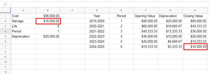
| Cost | $86,000.00 |
| Salvage (Scrap value) | $16,000.00 |
| Life (in years) | 6 |
| Period | 1 |
Formula:
=SYD(B1, B2, B3, B4)Result: $20,000.00 depreciation for Year 1.
Create a Depreciation Schedule with the SYD Function
To allocate depreciation across the asset’s life, create a table in the range E1:H, starting with the headers in E1:H1:
Period | Opening Value | Depreciation (SYD) | Closing Value
Fill the data as shown below:
| Period | Opening Value | Depreciation (SYD) | Closing Value |
|---|---|---|---|
| 1 | $86,000.00 | $20,000.00 | $66,000.00 |
| 2 | $66,000.00 | $16,666.67 | $49,333.33 |
| … | … | … | … |
- In
E2:E7, enter the periods—1 through 6. - In Column G, use the SYD function in Google Sheets to calculate depreciation for each year. Enter the following formula in cell
G2and drag it down toG7:
=SYD($B$1, $B$2, $B$3, E2)- In Column H (Closing Value), enter the following formula in
H2and drag it down toH7:
=F2 - G2To keep the flow of values:
- In
F2, enter the asset’s cost manually. - In
F3, use the following formula and drag it down:
=H2This setup will give you a complete SYD-based depreciation schedule year by year.
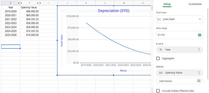
Create an SYD Depreciation Chart in Google Sheets
Once your depreciation table is ready, you can visualize it with a line chart.
Pre-step:
- In the range
D2:D8, enter the years in text format, such as:2019-2020,2020-2021, …2025-2026 - Copy the formula from
F7toF8to extend the data range for one more year.
Steps to Create the Chart:
- Hide column
E(Period column) to clean up the view. - Select the range
D1:F8. - Go to Insert > Chart.
- In the Chart Editor, change the chart type to Line chart.
Your SYD depreciation chart in Google Sheets is now ready!
Manual SYD Calculation in Google Sheets
If you want to calculate depreciation without using the SYD function, you can use the following formula:
= ((Cost − Salvage) × (Life − Period + 1) × 2) / (Life × (Life + 1))Using the earlier input values:
=((B1 - B2) * (B3 - B4 + 1) * 2) / (B3 * (B3 + 1))This also returns $20,000.00 for Period 1. Change the value in B4 to test different years and compare with the SYD function’s result.
Final Thoughts
The SYD function in Google Sheets is a practical choice when your assets lose value faster in their early years. It’s especially useful for machinery, vehicles, or any asset with front-loaded utility.
Use this function to create clear depreciation schedules and visual charts that align with your financial reporting or tax planning needs.


