Want to calculate the straight-line depreciation of your car, laptop, or any asset? The SLN function in Google Sheets makes it simple.
Straight-line depreciation is one of the most commonly used methods in accounting. It spreads the cost of an asset evenly over its useful life. In this tutorial, you’ll learn:
- What the SLN function does
- How to use SLN with examples
- How to manually calculate depreciation
- How to create a depreciation chart in Google Sheets
What Is the SLN Function in Google Sheets?
The SLN function calculates the depreciation of an asset for a single period using the straight-line method.
This is useful when you want to:
- Track the value of business assets over time
- Forecast depreciation for tax and accounting
- Create financial reports in Google Sheets
SLN Function Syntax
SLN(cost, salvage, life)Parameters:
cost: The initial purchase price of the assetsalvage: The expected value of the asset at the end of its useful life (residual value)life: The number of periods (usually years) over which the asset will be depreciated
SLN Example – Car Depreciation
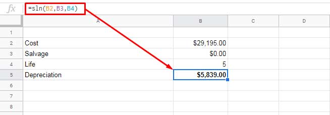
Let’s say you purchase a business car for $29,195 with a useful life of 5 years and expect no resale value (salvage = 0).
=SLN(29195, 0, 5)Result: $5,839
This means you’ll depreciate $5,839 every year.
Manual Depreciation Calculation in Google Sheets
If you prefer to calculate depreciation manually (without SLN), use:
=(cost - salvage) / lifeExample formula using cell references:
=(B2 - B3) / B4Where:
- B2 = $29,195 (cost)
- B3 = $0 (salvage)
- B4 = 5 (life)
This returns the same value as the SLN function: $5,839.
How to Create a Straight Line Depreciation Chart in Google Sheets
Step 1: Set Up the Depreciation Table in Google Sheets
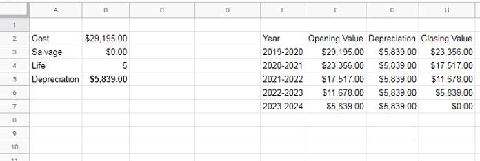
Start by creating the depreciation schedule in the range E2:H, beginning with the headers in row 2.
Enter the following column headers in E2:H2:
Year | Opening Value | Depreciation | Closing Value
Enter the first row of data:
| Year | Opening Value | Depreciation | Closing Value |
|---|---|---|---|
| Year 1 | =B2 | =$B$5 | =F3-G3 |
- In cell F3, enter
=B2to reference the asset’s original cost. - In G3, enter
=$B$5to fix the annual depreciation amount. - In H3, enter
=F3-G3to calculate the closing value for the first year.
Fill down for remaining years:
For Year 2 onward, follow this pattern:
| Year | Opening Value | Depreciation | Closing Value |
|---|---|---|---|
| Year 2 | =H3 | =$B$5 | =F4-G4 |
| Year 3 | =H4 | =$B$5 | =F5-G5 |
| … | … | … | … |
- In each row, the Opening Value equals the Closing Value of the previous year.
- The Depreciation remains fixed (use an absolute reference like
$B$5). - The Closing Value is calculated by subtracting depreciation from the opening value.
Drag the formulas in F4:H4 down as far as needed. For a 5-year depreciation period, extend the table through row 7.
Step 2: Insert the chart
- Select the table (e.g.,
E2:H7) - Go to Insert > Chart
- Set Chart Type to Line Chart
- Use “Year” as the X-axis and “Closing Value” as the Series
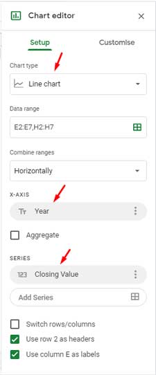
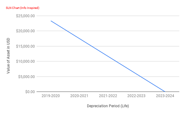
You’ll get a smooth downward-sloping line showing how your asset’s value drops over time.
SLN vs Other Depreciation Functions in Google Sheets
| Function | Method | Use Case |
|---|---|---|
| SLN | Straight-line | Even depreciation over time |
| SYD | Sum-of-years-digits | Accelerated depreciation |
| DDB | Double-declining balance | Higher depreciation in early years |
| DB | Declining balance | Similar to DDB but fixed rate |
| VDB | Variable declining balance | Custom range of depreciation periods |
| AMORLINC | Accounting-based method | Pro-rated depreciation (EU companies) |
👉 For more, check out: Google Sheets Functions Guide
FAQs About the SLN Function in Google Sheets
What is salvage value?
The salvage value (also called residual value) is the estimated value of an asset at the end of its useful life.
Does SLN work for partial years?
No. SLN only returns the depreciation for a full period. For partial depreciation or pro-rata calculations, use AMORLINC.
Can I use SLN for monthly depreciation?
Yes, just change the life parameter to represent the number of months instead of years.
Example: For a 5-year life, use life = 60 months.
=SLN(29195, 0, 60)Summary
The SLN function in Google Sheets is a reliable and easy way to compute depreciation using the straight-line method. It’s perfect for simple budgeting, accounting, and forecasting tasks.
Whether you’re managing a car fleet or calculating tax-deductible asset depreciation, SLN is the go-to formula.
Related Tutorials:


