The DB Function in Google Sheets uses the arithmetic declining balance method to find the depreciation of an asset.

You must understand the arithmetic declining balance since there are different methods followed in depreciation calculation.

You can check my financial functions to get other Google Sheets functions for depreciation.

Let’s start with Google Sheets DB Function syntax and a formula example. Then I’ll try to explain how to manually calculate the depreciation using the arithmetic declining balance method.

DB Function – Syntax and Arguments

Syntax:

DB(cost, salvage, life, period, [month])

Arguments:

• cost: It’s the initial cost of the asset.
• salvage: It’s the residual value of the asset (the value at the end of the depreciation).
• life: Asset’s useful life. It’s the number of periods over which the asset is depreciated.
• period: The (single) period for which we want to calculate the depreciation.
• month: The number of months (by default the function takes 12 months) in the first year of depreciation.

Example to the DB Function in Google Sheets

Sample Data:

In cell B5 you can use the below formula to calculate the depreciation using the arithmetic declining balance method.

=db(B1,B2,B3,B4)

The formula would return the DB as $196,500.00. This is for the 1st period.

In the formula, the number of months in the first year of depreciation is considered 12 months. This is because we have not specified the number of months (the ‘month’ parameter).

DB Formula which Includes the ‘Month’ Parameter:

=db(B1,B2,B3,B4,5)

Here in this formula, the number of period in the first year is 5 months. So the formula would return a much lesser amount as depreciation in the first period, i.e. $81,875.00.

Below you can read what happens behind the screen in the DB calculation.

Arithmetic Declining Balance Method in Google Sheets

We can use the below sample for learning the arithmetic declining balance.

In this method, except for the first period, we can use the following formula to calculate the depreciation of an asset.

Depreciation = (Initial Cost – Total Depreciation from Previous Periods) * Percentage of Depreciation

In this, the ‘Percentage of Depreciation‘ is equal to 1 – ((salvage / initial cost) ^ (1 / life)). Round this output to three digits.

For the first period, the equation is slightly different. Here is that equation for the first period.

Depreciation = Initial Cost * Percentage of Depreciation * Month/12

If we use the above sample data, the depreciation for the 1st period will be;

=50000*round(1-(5000/50000)^(1/5),3)*10/12

Result: $15,375.00

Here is the depreciation for the 2nd period:

=(50000-15375)*round(1-(5000/50000)^(1/5),3)

Result: $12,776.63

From the below screenshot, you can see that the DB function in Sheets returns the same above results for those periods.

I have copied the below DB formula in cell G2 to the cells down.

=DB($B$1,$B$2,$B$3,E2,$B$4)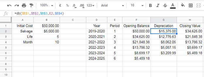

DB Line Chart in Google Sheets

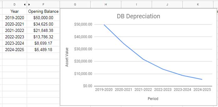
To create a DB line chart, use the above same data. But we don’t require the data in column E, so please hide it. We only need the data in the array D1:D7 and F1:F7.

Select the range D1:F7 and go to Insert > Chart. On the chart editor, select the chart “Line”.

Related Reading:

1. Google Sheets DDB Function in Depreciation Calculation.
2. How to Use the VDB Function in Google Sheets [Formula Examples].
3. SYD Function in Google Sheets for Accelerated Depreciation.
4. Google Sheets SLN Function in Straight Line Depreciation Calculation.
5. How to Use the AMORLINC Function in Google Sheets.