The VDB function in Google Sheets uses the double declining balance method to calculate depreciation for a given start and end period. In this financial function, you can specify the starting and ending period to get the depreciation during that period.
For example, if the useful life of an asset is 10 years, you can find the depreciation of that asset for the periods 1 to 5 or 2 to 6 and so on.
If you want to find the depreciation for any specific period, single year normally, then simply use the DDB function as both of the functions follow the double declining balance method.
I have already given ample information on the double declining balance method in my post here – Google Sheets DDB Function in Depreciation Calculation. So I am not going into that details again.
Depreciation Calculation Using Variable Declining Balance (VDB) Method
Before proceeding further, you must know the DDB calculation. That prompts me to give you an idea about DDB in a nutshell.
To understand DDB you must know the Straight Line depreciation (SLN). In SLN the percentage of depreciation will be the same in all the useful life period.
You can get that percentage by dividing 100% by the useful life of the asset in years. If the (useful) life of an asset (equipment) is 10 years, the calculation will be =100%/10 or you can simply use 1/10. You will then get 0.10 means 10%.
Example:
In the following formula, the asset value is 100,000 and the scrap value (salvage) is 10,000. Then the depreciation amount will be 9,000 each year.
=(100000-10000)*10%In DDB, the depreciation percentage will be just double of the above SLN percentage. That means 20%. But that doesn’t mean the depreciation will be just double of the straight line method, i.e. 18,000.
Here unlike SLN, you must not deduct the scrap value (salvage) from the cost of asset.
=100000*20%Result: 20,000
Here also the percentage will be the same during the useful life of the period. But the depreciation value will be declining! How?
For the second year, the depreciation value will be 16,000. The below formula reveals this.
=(100000-20000)*20%In this 100,000 is the cost of the asset, 20,000 is the depreciation amount of the first year. Hope you can understand this.
Google Sheets VDB Function – Syntax and Formula Examples
Syntax of the VDB Function in Google Sheets
VDB(cost, salvage, life, start_period, end_period, [factor], [no_switch])Let me explain the arguments.
cost – the initial asset cost.
salvage – scrap value (the value of the asset at the end of its useful life period).
life – the useful life of the asset.
start_period – the period from.
end_period – the period to.
factor – optional and 2 (double declining) by default.
no_switch – it (TRUE/FALSE) determines whether to switch to straight-line depreciation (default by FALSE) when the SLN depreciation is greater than the declining balance calculation.
VDB Formula Example in Sheets
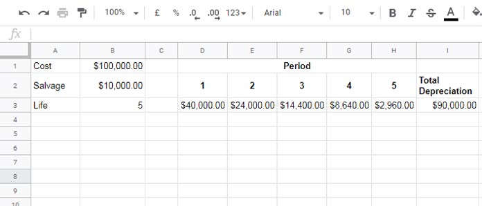
See the sample data given in the range B1:B3. Just leave the other values for the time-being.

With the help of the VDB function, you can find the depreciation amount for each period as below.
=vdb(B1,B2,B3,0,1,2,FALSE)In this VDB formula you know the values in the cells B1, B2, and B3. The number 0 represents start period and 1 represents end period. The number 2 represents the factor.
Then to calculate the depreciation for the second period, you can use the formula as below.
=vdb(B1,B2,B3,1,2,2,FALSE)But the main purpose of the VDB function in Google Sheets is not the above. The above calculation you can simply do with the below DDB formulas.
First Period:
=DDB($B$1,$B$2,$B$3,1)Second Period:
=DDB($B$1,$B$2,$B$3,2)Then what is the difference between DDB and VDB functions in Google Sheets?
VDB vs. DDB in Google Sheets
To calculate the depreciation amount for the above two periods, you can use a single VDB formula as below.
=vdb(B1,B2,B3,0,2,2,FALSE)Take a look at the above screenshot. I have the following DDB formula in cell D3 which dragged to the right.
=DDB($B$1,$B$2,$B$3,D2)When you drag the formula right, the cell reference D2 changes to E2, F2 … as it is relative cell reference and other references in the formula are absolute (refer this guide for more details – Placement and Use of Single/Double Dollar Symbols in Formulas.
In cell I3 you can see the total depreciation during the useful life of the asset (cost-salvage). It’s the sum of the values in the array/range D3:H3.
Using VDB you can find the total depreciation from the start to end as below.
=vdb(B1,B2,B3,0,5,2,FALSE)In this VDB formula, 0 is the start_period and 5 is the end_period and as you know the useful life span of the asset is 5 years.


