The Google Sheets DDB function is categorized under financial functions and is used to calculate the accelerated depreciation of an asset. Accelerated depreciation allows for a larger depreciation expense in the earlier years of an asset’s life, which is advantageous for companies looking to reduce taxable income during that time.
Why Companies Prefer Accelerated Depreciation
In accelerated depreciation, the depreciation amount is higher in the initial years of an asset’s life and decreases over time. This method is often preferred because it allows companies to offset higher expenses earlier, reducing their taxable income in those initial years.
As you may know, the SYD function is also used to calculate accelerated depreciation. I have already detailed the use of the SYD function in a previous tutorial (linked here). The SYD method (Sum-of-Years-Digits) distributes depreciation costs more heavily in the early years of an asset’s useful life.
Syntax of the Google Sheets DDB Function
DDB(cost, salvage, life, period, [factor])The DDB function follows a similar structure to other depreciation functions in Google Sheets, making it easy to understand its arguments. The first three arguments—cost, salvage, and life—are common across most depreciation formulas.
- cost: The initial cost of the asset that you want to depreciate.
- salvage: The asset’s residual (or scrap) value, which is its expected value at the end of its useful life.
- life: The useful life span of the asset, representing the number of periods over which the asset will be depreciated.
- Period: The single period within life for which to calculate depreciation.
- factor: The rate at which depreciation decreases. This is optional and defaults to 2, representing the double-declining balance method.
Note: In contrast, the SYD function (another accelerated depreciation method) does not include a “factor” argument.
How to Use the DDB Function in Google Sheets
Here’s an example illustrating how to use the DDB function in Google Sheets.
| A | B |
| Cost | $10,000.00 |
| Salvage (Residual/Scrap Value) | $1,000.00 |
| Life (Useful Life) | 5 |
| Period | 1 |
Formula:
=DDB(B1, B2, B3, B4)In the above example, the DDB function calculates the depreciation amount for the 1st period (year) using the Double Declining Balance (DDB) method, which equals $4,000.00.
The useful life of this asset is 5 years, and the formula shows the depreciation for the first period. To calculate the depreciation for the remaining periods, you can drag the formula down, as shown below.
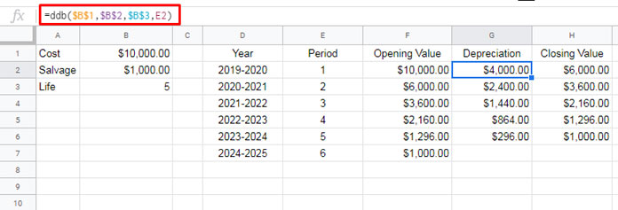
In the DDB formula in cell G2, you take the values for cost, salvage, and life from cells B1, B2, and B3, respectively. The value for ‘period’ comes from cell E2. When you drag the formula down, it updates the period based on cells E3, E4, and so on, as you use relative cell references for the period while keeping the other cell references absolute.
Alternatively, you can use this array formula:
=ArrayFormula(DDB($B$1, $B$2, $B$3, SEQUENCE(5)))This avoids using the helper range E2:E5, which contains sequence numbers from 1 to 5.
Understanding Double Declining Balance Calculation
Before understanding Double Declining Balance (DDB) depreciation, it’s useful to know how Straight-Line Depreciation (SLN) works.
The formula for Straight-Line Depreciation is:
SLN = (cost – salvage) / lifeFor example, if you use the same input values from the DDB formula above, the SLN calculation would be:
=(10000 - 1000) / 5 = $1,800.00You can also use the built-in SLN function in Google Sheets:
=SLN(10000, 1000, 5)The result is $1,800.00, which represents 20% of the asset’s depreciable value (cost-salvage). This means that using the Straight-Line Depreciation method, the asset will depreciate by 20% each year, for a total of 5 years.
Comparing SLN and DDB Depreciation
The Double Declining Balance (DDB) method doubles the depreciation percentage. For this example, the percentage would be 40% per year. However, unlike SLN, the depreciation amount is not constant each year—it decreases as the book value of the asset decreases.
For the first year, the calculation is:
Depreciation = $10,000 * 40% = $4,000.00For the second year, the calculation is:
Depreciation = ($10,000 - $4,000) * 40% = $2,400.00This process continues for each subsequent year, with the depreciation percentage applied to the remaining book value of the asset.
VDB Function
For your information, the VDB function also calculates depreciation using the double-declining balance method. However, it is more flexible than the DDB function, as it allows you to specify a start period and end period to calculate depreciation across a range of periods.
DDB Depreciation Chart in Google Sheets
You can easily visualize the results of the DDB function by creating a line chart in Google Sheets.
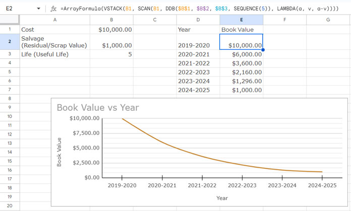
Enter the years of depreciation in column D (D1:D7), starting with the label “Year” in cell D1.
Enter the label “Book Value” in cell E1. Then, enter the following formula in cell E2, which calculates the remaining book values of an asset over its useful life by subtracting the depreciation amounts from the initial cost and stacking the results vertically:
=ArrayFormula(VSTACK(B1, SCAN(B1, DDB($B$1, $B$2, $B$3, SEQUENCE(5)), LAMBDA(a, v, a-v))))Select the range D1:E7 and click Insert > Chart. In the Chart Editor, change the chart type to Line, and you’re done!
That’s all about the DDB function in Google Sheets. Try it out, and enjoy the simplicity of calculating accelerated depreciation!


