This tutorial explains how to return the sum instead of Min or Max in the Pivot Table Grand Total row in Google Sheets.
This article is part of the Pivot Table Calculations & Advanced Metrics hub, which explores advanced pivot table calculations and reporting techniques in Google Sheets.
Understanding the Issue
When you use MAX or MIN in the Values field of a Pivot Table, the Grand Total row also applies the same function. Instead of summing the Min or Max values from each group, it returns the overall Min or Max of that column.
For example, consider this sample data:
| Date | Item | Receipt |
| 13/10/21 | Product 1 | 20 |
| 13/10/21 | Product 1 | 5 |
| 14/10/21 | Product 1 | 10 |
| 14/10/21 | Product 1 | 9 |
| 13/10/21 | Product 2 | 30 |
| 13/10/21 | Product 2 | 31 |
| 14/10/21 | Product 2 | 19 |
| 14/10/21 | Product 2 | 25 |
Now, assume the Pivot Table settings are as follows:
- Rows: Item (with “Show Totals” enabled)
- Values: Receipt (Summarized by MIN)
The output would be:
| Item | MIN of Receipt |
| Product 1 | 5 |
| Product 2 | 19 |
| Grand Total | 5 |
The Issue
Instead of summing the Min values (5 + 19 = 24), the Pivot Table shows 5, which is just the lowest value in the column. The same issue occurs if you use MAX, where the Grand Total will display the highest value instead of the sum of Max values.
Fix: Get Sum Instead of Min in Pivot Table Grand Total
Since there’s no built-in option to change how the Grand Total is calculated, we can use a helper column in the source data.
Step 1: Add Helper Columns
Assume your sample data is in A1:C in Sheet1.
- In D1, enter the field label for the helper column, e.g., Helper.
- In E1, enter another field label, e.g., Helper2.
- In E2, create a group identifier:
- If grouping by Item,
=ArrayFormula(B2:B)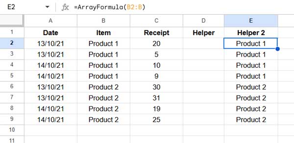
- If grouping by Date & Item,
=ArrayFormula(B2:B&A2:A)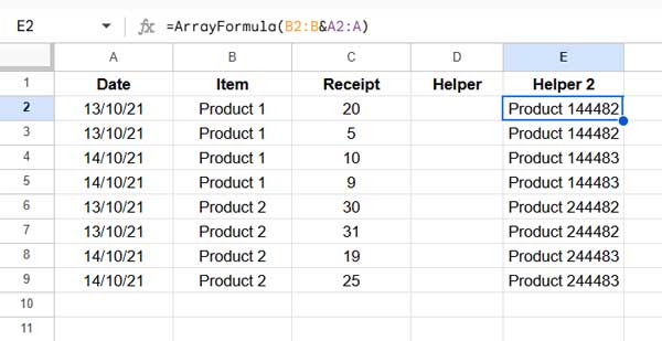
- If grouping by Item,
Step 2: Calculate the Min Value for Each Group
In D2, enter the following formula to return the Min value at each group change:
=MAP(E2:E, LAMBDA(cat, ARRAYFORMULA(IF(COUNTIFS(E2:E, cat, ROW(E2:E), ">="&ROW(cat))=1, MINIFS(C2:C, E2:E, cat),))))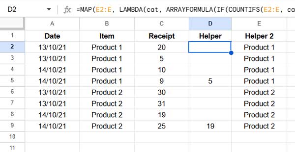
Where:
C2:C: The column containing the values for which the minimum is calculated (e.g., “Receipt” column).E2:E: The helper column used for grouping.
Note: Sorting the data is not necessary for the formula to work. However, sorting the grouping columns (e.g., sorting by Item or Item and Date) will make it easier to read and interpret the formula results in column D.
Step 3: Create the Pivot Table
- Select A1:E and go to Insert > Pivot Table.
- Click Create to generate a new sheet with the Pivot Table.
- Set up the Pivot Table:
- Rows: Drag and place Item.
- Values: Drag and place Helper and select SUM instead of MIN.
- (Optional) Filter: Add Item and apply “Is not empty”.
- Click B1 in the Pivot Table and rename SUM of Helper to Min of Receipt.
The corrected output:
| Item | Min of Receipt |
| Product 1 | 5 |
| Product 2 | 19 |
| Grand Total | 24 |
Fix: Get Sum Instead of Max in Pivot Table Grand Total
For the Max scenario, follow the same steps, but in D2, replace MINIFS with MAXIFS:
=MAP(E2:E, LAMBDA(cat, ARRAYFORMULA(IF(COUNTIFS(E2:E, cat, ROW(E2:E), ">="&ROW(cat))=1, MAXIFS(C2:C, E2:E, cat),))))Optional: Using a Named Function
To simplify the formula in D2, you can use a custom Named Function instead of writing the full formula.
- For Min values, use:
=IFNA(MIN_AT_EACH_CHANGE(group_range, subtotal_range, mode)) - For Max values, use:
=IFNA(MAX_AT_EACH_CHANGE(group_range, subtotal_range, mode))
Replace group_range with E2:E, subtotal_range with C2:C, and set mode to -1.
You can import these Named Functions from AT_EACH_CHANGE Named Functions for Group Totals in Sheets for easy implementation.
Conclusion
We have explored a workaround to return the sum instead of Min or Max in Pivot Table Grand Total in Google Sheets. The approach involves:
- Using helper columns to track group changes.
- Applying MINIFS or MAXIFS to extract the correct values.
- Summarizing the helper column using SUM in the Pivot Table.
This method also supports multi-level grouping by including additional columns in the helper field.


