Show Rolling 7, 30, 60 Day Data in a Pivot Table in Google Sheets

Want your Pivot Table to always show the latest 7, 30, or 60 days of data without constantly opening the editor? Here’s a neat trick using a helper cell and a simple formula to keep things dynamic. Once set up, all you need to do is change a number, and your Pivot Table updates like magic.

Table of Contents

The Idea in a Nutshell

We’ll set this up using:

A helper cell to type in how many days back you want to see (7, 30, 60, etc.)
An ArrayFormula that marks rows as TRUE or FALSE depending on whether they fall within that range
A Pivot Table filter or Slicer that includes only the TRUE rows

So anytime you change the number in the helper cell, your Pivot Table automatically shows only the latest n days—no need to dig into the editor.

Rolling 7, 30, or 60 day data dynamically updating in Pivot Table in Google Sheets

This guide belongs to the Pivot Table Calculations & Advanced Metrics hub—your reference for advanced pivot table calculations in Google Sheets.

Let’s Set It Up: Rolling Days in a Google Sheets Pivot Table

Here’s how to show rolling 7, 30, or 60-day data in a Pivot Table.

Step 1: The Source Data

In the Source sheet, we’ve got the usual stuff:

Column A: Dates
Column B: Values (or any other metric)

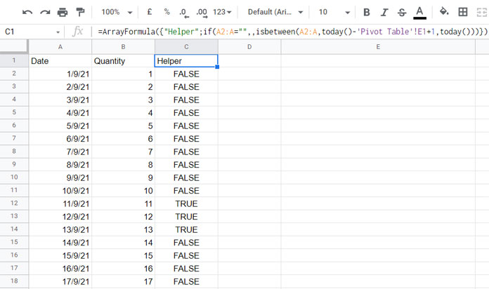
We’ll add a third column (C) to help us filter. This column will return TRUE if the row’s date is within the rolling range you specify.

That rolling range comes from a helper cell—E1 in the “Pivot Table” sheet. Whatever number you put there (say 30), the formula in column C will return TRUE for rows from the last 30 days (including today), and FALSE otherwise.

Here’s what you put in Source!C1:

=ArrayFormula(
  {"Helper";
    IF(
      A2:A = "",,
      ISBETWEEN(A2:A, TODAY() - 'Pivot Table'!E1 + 1, TODAY())
    )
  }
)

Helper column showing TRUE/FALSE results for rolling n-day data in Pivot Table setup

A quick breakdown:

A2:A = "" skips any blank rows
ISBETWEEN(...) checks whether the date is within the range from today back to n days ago
"Helper" becomes the name you’ll use to filter in the Pivot Table or Slicer

So if you enter 30 in 'Pivot Table'!E1, this formula marks all dates from the last 30 days as TRUE.

Step 2: The Helper Cell

In the “Pivot Table” sheet, cell E1 is where you type how many days you want to look back—7, 30, 60, or even a custom number.

Change the number, and your data updates automatically. Simple and flexible.

Quick Recap of the Formula

Here’s what’s going on inside that formula:

IF(A2:A = "", , …) – keeps blanks out of the way
ISBETWEEN(A2:A, TODAY() - 'Pivot Table'!E1 + 1, TODAY()) – checks if each date is within the last n days
Rows marked TRUE get picked up by the Pivot Table or Slicer

Step 3: Filter the Pivot Table

If you’re not using a Slicer, here’s how to filter directly inside the Pivot Table:

Open the Pivot Table editor by clicking the pencil icon that appears when you hover over the Pivot Table report.
Under Filter, click Add and select the Helper column
Uncheck FALSE and Blanks so only TRUE rows show up
Click OK

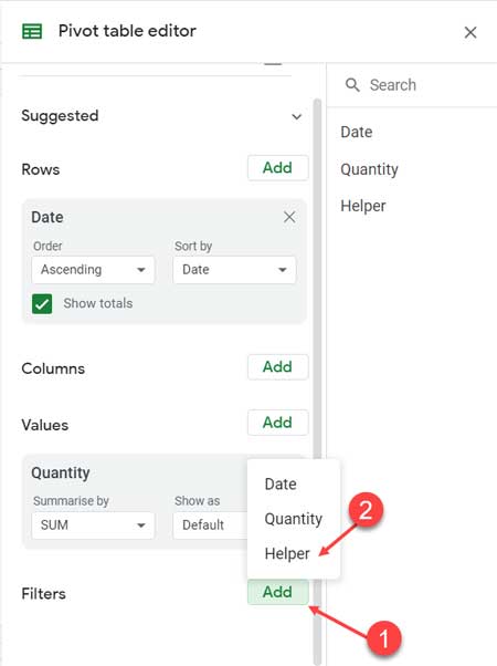
Pivot Table filter set to include only TRUE values from the helper column

Done! Your Pivot Table now shows only the rows from the last n days, based on what you enter in E1.

Optional: Use a Slicer Instead

Prefer a Slicer? You can do that too:

Click anywhere inside your Pivot Table (e.g., cell A1)
Go to Data > Add a Slicer
In the Slicer panel:
- Set the column to Helper
- Set the range to Source!A1:C
Click the Slicer dropdown on the sheet and uncheck FALSE and blanks
Apply it

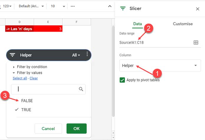
Slicer settings filtering data using TRUE values from the helper column

Now your Pivot Table is filtered dynamically using the Slicer instead.

Sample Sheet

Wrap-Up

And that’s it! With this setup, you can show rolling 7, 30, or 60-day data in a Google Sheets Pivot Table—no manual filtering or editing formulas each time. Just change the number in your helper cell and let Google Sheets do the rest.

Thanks for reading—and enjoy your streamlined reporting!