To calculate quartiles based on conditions, referred to as “Quartile IF,” we will use a combination of formulas in Google Sheets.

Sometimes, you may want to calculate quartiles based on specific conditions, such as the quartile of test scores for students who scored above a certain threshold, or values that fall within specific date ranges, months, or years.

The QUARTILE function does not accept criteria, and there is no QUARTILEIF function available in Google Sheets. Therefore, we resort to workarounds that involve the FILTER function.

We will filter the values based on conditions using FILTER, and for that, we can also use QUERY. Another option is the IF function. We will explore all these varieties in this tutorial.

Quartile IF Analysis in Google Sheets

In the following example, I have student names in column A and their test scores in column B. Let’s find quartiles 0 to 4 of test scores above 70. Please note that we will use the range B2:B as B1 contains the field label.

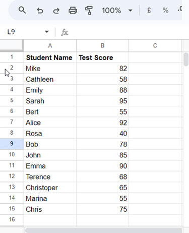
In Quartile IF, the logic is to extract the values that fall within the threshold limit, where in this case, the test scores are greater than or equal to 70.

The following formula can be used to extract the values that fall within the threshold limit:

=FILTER(B2:B, B2:B>=70)

In the above FILTER formula, the range to filter is B2:B, and the condition is B2:B>=70. You just need to wrap it with the QUARTILE function and specify the quartile number to get the quartile:

=QUARTILE(FILTER(B2:B, B2:B>=70), 3)

The above formula will return the third quartile. If you want to get quartiles 0, 1, 2, 3, and 4 in one go, specify the quartile numbers as an array and enter the formula as an array formula:

=ArrayFormula(QUARTILE(FILTER(B2:B, B2:B>=70), HSTACK(0, 1, 2, 3, 4)))

Result: {75, 81, 86.5, 90.5, 95}

In this formula, we have used the HSTACK function to create a one-dimensional horizontal array of quartile numbers. If you want the result vertically, replace HSTACK with VSTACK.

FILTER Replacement:

QUERY: QUERY(B2:B, "SELECT B WHERE B>=70", 0)

IF: =ArrayFormula(IF(B2:B>=70, B2:B))

Quartile IFs Analysis in Google Sheets

In the above examples, we have specified one condition, i.e., test score >=70. Here, let’s see how to calculate Quartile IFs with multiple conditions.

Here, we have dates in column A and numeric values in column B.

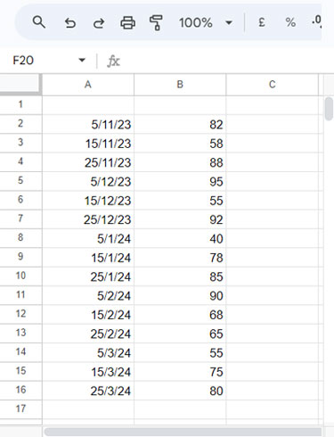
How do we calculate the second quartile in a specific year, for example, 2024?

The following FILTER formula filters column B if the year in column A falls in 2024:

=FILTER(B2:B, YEAR(A2:A)=2024)

In this FILTER formula, the range to filter is B2:B, and the criterion is YEAR(A2:A)=2024. The YEAR function extracts the year from the date.

Wrap it with the QUARTILE function as below:

=QUARTILE(FILTER(B2:B, YEAR(A2:A)=2024), 2)

This is still an example of Quartile IF as it holds one criterion. What about multiple conditions Quartile IFs?

For example, we need to filter the dates that fall in the years 2023 and 2024 and find the quartile. We can use either of the below FILTER formulas for that:

=FILTER(B2:B, (YEAR(A2:A)=2023)+(YEAR(A2:A)=2024))
=FILTER(B2:B, ISBETWEEN(YEAR(A2:A), 2023, 2024))

Wrap it with QUARTILE and specify the quartile number.

Additional Tips

What about Quartile IFs with a date range?

The following formula answers this:

=FILTER(B2:B, A2:A>=DATE(2024, 1, 1), A2:A<=DATE(2024, 2, 29))

It filters the data that falls between January 1, 2024, and February 29, 2024.

Notes:

• In the above formula, the date is specified in the DATE function syntax DATE(year, month, day).
• In date range formulas, whenever you want to specify month-end dates such as DATE(2024, 2, 29) in the above example, I suggest using EOMONTH(DATE(2024, 2, 1), 0) which converts the beginning of the month date to the end of the month date and ensures we are using the correct month-end date.

Conclusion

To master Quartile IF, it’s essential to become proficient with either the FILTER function or the IF function. This mastery enables you to filter values based on conditions, which can then be utilized within the QUARTILE function.

For more advanced filtering capabilities, consider using QUERY. All these functions are available for learning within my function guide.

You may also be interested in: How to Calculate the Interquartile Range (IQR) in Google Sheets.