


We can use multiple search strings in a single SEARCH function/formula in Google Sheets. No need to nest the SEARCH function to do multiple searches.
Nested search is about using the SEARCH function in a nested way in Google Sheets to incorporate more than one search string.
For example, a supplier has sent us the following items.
| Date | Despatched Items |
| 01/01/2020 | Apple – 100 kg and Orange 50 kg. |
I want to test if either of the items “Apple” or “Banana” is available on the despatched list.
The formula would be like this for a single item.
=isnumber(search("Apple","Apple - 100 kg and Orange 50 kg."))In the nested approach (which is not recommended though), for searching the availability of two items, the will be something like this.
=or(isnumber(search("Apple","Apple - 100 kg and Orange 50 kg.")),isnumber(search("Banana","Apple - 100 kg and Orange 50 kg.")))The OR logical function would return TRUE if either of the items is available.
Note: To learn OR, SEARCH, or other popular Google Sheets functions please check my Google Sheets Function Guide.
What’s the alternative to the so-called nested SEARCH function then?
I’ll come to that. Before I should explain why I have used ISNUMBER with SEARCH in the example above.
The Role of ISNUMBER with SEARCH Function in Google Sheets
Have you noticed the use of ISNUMBER with SEARCH in the formulas above?
The Search function in Google Sheets is for searching a single text string. It returns not TRUE or FALSE but the position at which the text string is first found within the text.
If cell A2 contains the string “Work allocated to Ben and John” the formula =search("Ben",A2) will return 19.
Note: The SEARCH function doesn’t consider whether the text is in upper/lower/proper case as it’s case insensitive.
When there is no match the formula would return #VALUE! error. To remove that error, we can use ISNUMBER together with SEARCH.
The ISNUMBER will convert the error value(s) to Boolean FALSE value(s) and the matching position to TRUE.
=isnumber(search("Ben",A2))
or
=--isnumber(search("Ben",A2))
The first formula would return TRUE (not 19) whereas the second formula would return 1 (Boolean TRUE is equal to 1, and FALSE is equal to 0).
A Single SEARCH Formula for Multiple Searches in Google Sheets
Let’s see how to use multiple search strings in a single SEARCH function in Google Sheets without nesting it.
If you go through the SEARCH function syntax, you can understand that there is no way to include multiple search strings (search_for).
SEARCH(search_for, text_to_search, [starting_at])Note:- starting_at is an optional argument.
No search_for_1, search_for_2 in the syntax. But the fact is that you are free to use multiple search texts in search_for. How?
Syntax:
Sum(ArrayFormula(--Isnumber(SEARCH({search_for_1, search_for_2, search_for_3,... },text_to_search))))If we follow the above fruit example, the nested SEARCH formula can be replaced by the below single SEARCH formula.
=Sum(ArrayFormula(--Isnumber(SEARCH({"Apple","Banana"},"Apple - 100 kg and Orange 50 kg."))))Note: If the formula returns 0, that means the SEARCH could not find any match. If it returns >0, then;
1 = 1 match
2 = 2 matches and so on.
Search to Find If the Cell Contains One of Many Things in Google Sheets
The same above example but here replacing search_for and text_to_search arguments with corresponding cell references.
The SEARCH formula to find if the cell A2 contains one of many things (C2:C3):
=Sum(ArrayFormula(--Isnumber(SEARCH({C2,C3},A2))))
or
=Sum(ArrayFormula(--Isnumber(SEARCH(C2:C3,A2))))
Multiple Search_For and Multiple Text_To_Search in a Single SEARCH Formula
We have seen above how to use multiple search strings (multiple search_for) in a single SEARCH formula in Google Sheets. Now let me take you one step further!
In addition to the above, below we can learn how to use multiple text_to_search (range/array) with SEARCH.
I have two (each) non-array and array formulas for you to choose from. Let me start with the non-array formulas first.
Actually, the non-array formulas do not justify the title as it only uses a single text_to_search. We need to manually drag/copy the formula for additional text_to_search.
Then why I am starting with or providing you the non-array formula?
The reason is simple. It is the same formula that we have used above to find if a cell contains one of many things. Here is an example.
Non-Array Search Formula with Multiple Search Text
The following formula in cell D6 is copy-pasted to the range D7:D12.
=Sum(ArrayFormula(--Isnumber(SEARCH($C$2:$C$4,B6))))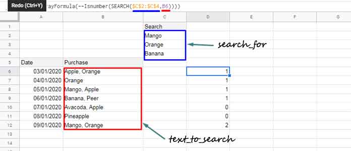
I am not repeating the formula explanation.
An alternative formula, that is common among Excel users, is below.
=sumproduct(isnumber(search(transpose($C$2:$C$4),B6)))Array Search Formula with Multiple Search Text
We must replace (as far as I’m concerned) non-array formulas with an array formula, wherever possible in Google Sheets. It has several benefits but I am leaving that topic this time.
Using MMULT with SEARCH we can use more than one search strings (search_for) that are also in a range (multiple text_to_search) in a single SEARCH Formula in Google Sheets.
Note:- There are other two functions – SEQUENCE and TRANSPOSE – that are also involved, but MMULT is the key.
Formula to enter in cell D2 which will automatically expand to down:
=ArrayFormula(mmult(--isnumber(search(transpose(C2:C4),B6:B12)),sequence(3,1)^0))In this C2:C4 contains the search_for strings, B6:B12 contains the text_to_search strings.
The number 3 in Sequence represents 3 rows (the count of the cells in the range C2:C4) and the number 1 represents one column.
Other than C2:C4 and B6:B12, you only need to take care of the number of rows (here 3) in Sequence. It should match the count of cells in the search_for range.
Replacing SEARCH ArrayFormula with REGEXMATCH ArrayFormula in Google Sheets
In all the above examples, the SEARCH formula (no matter whether it’s in an array or non-array form) returns the count of match. But the Regexmatch will return TRUE/FALSE based on match/mismatch. The below image is self-explanatory.
=ArrayFormula(regexmatch(lower(B6:B12),join("|",true,lower(C2:C4))))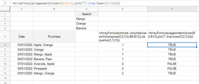
For the above Regex formula explanation, please read this post – Match Two Columns that Contain Values Not in Any Order Using Regex.
That’s all, Enjoy!
I’m looking to search column ‘B’. If it contains ‘-ch’, I want it to say ‘chiffon’. If it contains ‘-rs’, I want it to say ‘raw silk’. If it contains ‘-ss’, I want it to say ‘silk’, plus about 5 more.
I’ve tried:
=IFS(ISNUMBER(SEARCH("-CH",B3)),"CHIFFON",(SEARCH("-SC",B3)),"Silk Crepe",(SEARCH("-SS",B3)),"Silk",(SEARCH("-GD",B3)),"GOLD")
It only seems to apply for the first couple, i.e., chiffon and silk crepe, and then after that stops searching.
Any suggestions?
Hi, here is the corrected formula:
=IFS(ISNUMBER(SEARCH("-CH",B3)),"CHIFFON",
ISNUMBER(SEARCH("-SC",B3)),"Silk Crepe",
ISNUMBER(SEARCH("-SS",B3)),"Silk",
ISNUMBER(SEARCH("-GD",B3)),"GOLD"
)
You can also try this version, in which you can add more search terms:
=FILTER(HSTACK("CHIFFON", "Silk Crepe", "Silk","GOLD"),
IFERROR(SEARCH({"-CH", "-SC", "-SS", "-GD"}, B3))
)
Hi Prashanth,
My data is:
FALC
FYLC
RETA
N6LK
AVDE
M1LG
GDRZF
VASO
F1LS
DO
CMT
I want to identify those cells that have a number in it (0 to 9). How do I do that? I tried using the array formula, but I was unable to replicate your results.
Thanks.
Hi SPH,
Nice to see you again!
You can use the REGEXMATCH and ARRAYFORMULA functions to do this.
For example, the following formula will return an array of TRUE or FALSE values, indicating whether each cell in the range A1:A100 contains a number:
=ArrayFormula(REGEXMATCH(A1:A100,"[0-9]"))Hi Prashanth,
How can you return the index of the match (if you are only looking for a single search substring)?
Currently, your formula returns the COUNT of matches in the range.
Hi, Mohammed,
Try the XMATCH function. Here is one example.
=xmatch("*apple*",C:C,2,1)This formula is for partial match “apple” in column C.
Would it be possible to search for phrases inside another google doc document with this technique, or does it only work inside Google Sheets’ cells and cell ranges? Thank you.
Hi, Mario,
Nope! That’s not supported.
Thanks.
Is there a way to do multiple finds on a cell rather than nesting FIND formulas as in this example:
=if(not(iserr(find("500m",C16))),"500m",if(not(iserr(find("1km",C16))),"1km",
if(not(iserr(find("250m",C16))),"250m",
if(not(iserr(find("MCD",C16))),"Combined","N/A"))))
Hi, Michael,
It seems you not only want multiple finds but also to extract them.
In that scenario, try REGEXEXTRACT.
=IFNA(REGEXEXTRACT(C16,"(?i)500m|1km|250m|MCD"),"N/A")