I know there are already formulas available on the web to find the most frequently occurring text string, which we can call the Mode, in a list. But what about finding multiple Modes of text values in Google Sheets?
Sometimes, there may be two or more most frequently occurring texts in a list. I have a Google Sheets formula that you can use to find the MODE as well as MODE.MULT for text strings.
As you may know, we can’t use the MODE function to find the Mode of non-numerical values. Similarly, we can’t use the MODE.MULT function to return multiple Modes of non-numerical values. Both are statistical functions designed for numerical data.
So, how can we find the Mode of text values in Google Sheets?
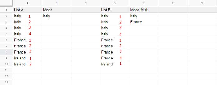
Consider the list in column A below. The Mode of text is “Italy,” as it repeats 4 times, which is more than any other text value in that list.
But in the list in column D, the strings “Italy” and “France” each repeated four times. Therefore, both these text values are the most frequently occurring text values (multiple Modes) in this list.
Formula to Find the Mode of Non-Numeric Values in Google Sheets
My formula will work in both cases, returning single as well as multiple Modes, without any modification.
Formula to Find the Mode/Modes of Text Strings in Google Sheets:
=ArrayFormula(LET(
   range, A2:A,
   rp, IFERROR(MATCH(range, range, 0)),
   mm, MODE.MULT(rp),
   XLOOKUP(mm, rp, range)
))
This formula is designed to work with the list in column A (range A2:A). If your list to find the Mode is in any other column, please modify the cell references in the formula accordingly.
Tip: If you are using the data in a table, feel free to replace A2:A with a structured reference, such as Table1[Country], where Table1 is the table name and Country is the column specifier in the table. You can read more about it here: Structured Table References in Formulas in Google Sheets.
How Does the Formula Find the Most Frequently Occurring Strings in Google Sheets?
I understand that simply presenting a complex-looking formula might not suffice for everyone. Some of you may be curious about how the formula identifies the most frequently occurring text string from a list.
In my formula, I’ve utilized several functions. I’ll attempt to explain the role of each function used in the simplest way possible.
MATCH to Return the Relative Position of All the Text Strings in the List
In cell B2, enter this MATCH formula.
Formula 1:
=ArrayFormula(MATCH(A2:A, A2:A, 0))This adheres to the syntax ArrayFormula(MATCH(search_key, range, search_type)).
Where:
search_key: A2:Arange: A2:Asearch_type: 0
We have used the ARRAYFORMULA function since we use multiple search keys to match.
It will return the relative position of each item in the range A2:A based on their first occurrence within that range.
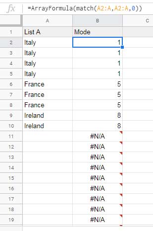
For example, “Italy”, “France”, and “Ireland” are the three unique values in the list in A2:A.
The relative position of the text “Italy” is 1 as it is in the first row in the range A2:A. The relative position of the text “France” is 5 as it’s in the fifth row in the range A2:A.
Take a look at the relative position of the string “Ireland”, and you can see that it’s 8.
We will use these relative positions to find the Mode of text values.
We have converted the text strings to numbers because the MODE.MULT function can only operate on numeric data, not text.
The Role of the MODE.MULT Function in Finding the Most Frequently Occurring Text Values
After entering the MATCH formula above, we have a few numbers in column B, right?
What we want is to find the Mode of those numbers. For that, you can use MODE or MODE.MULT in cell C2.
I prefer the MODE.MULT function as it can return multiple Modes.
Use the above same MATCH formula within MODE.MULT, but include the IFERROR function to remove N/A error values.
Formula 2:
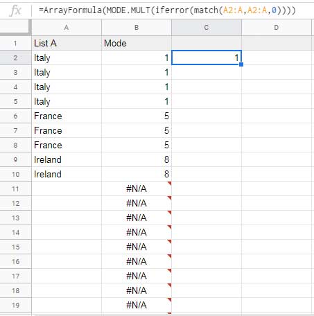
=ArrayFormula(MODE.MULT(IFERROR(MATCH(A2:A, A2:A, 0))))It follows the syntax ArrayFormula(MODE.MULT(value)), where the value is the output returned by formula #1.
The formula returns 1, which corresponds to the most frequently occurring relative position.
XLOOKUP to Lookup Multiple Modes of Matches and Return Corresponding Texts
We will look up the output of the Step #2 formula (MODE.MULT result) in the Step #1 formula output (MATCH result) and return country names from the matching rows from A2:A. We will use XLOOKUP for that.
=ArrayFormula(XLOOKUP(C2, B2:B, A2:A))This adheres to the syntax ArrayFormula(XLOOKUP(search_key, lookup_range, result_range)).
Where:
search_key: C2 (MODE.MULT result)lookup_range: B2:B (MATCH result)result_range: A2:A
Replace C2 and B2:B with the corresponding formulas:
=ArrayFormula(XLOOKUP(
   MODE.MULT(IFERROR(MATCH(A2:A, A2:A, 0))),
   MATCH(A2:A, A2:A, 0),
   A2:A
))
This is the formula to get the Mode of text values in Google Sheets.
In our original formula, we used the LET function to avoid repeated calculation of MATCH by naming it with ‘rp’ (represents relative position), A2:A with ‘range’, and MODE.MULT with ‘mm’. That makes the formula more efficient and reader-friendly.
Conclusion
The above method is not the only way to obtain the Mode of text values. You can also achieve this by using a combination of QUERY and SORTN.
Example:
=SORTN(QUERY({A2:A}, "SELECT Col1, COUNT(Col1) WHERE Col1 IS NOT NULL GROUP BY Col1 ORDER BY COUNT(Col1) DESC LABEL COUNT(Col1)'' ", 0), 1, 1, 2, 0)In this formula, the QUERY function calculates the count of occurrences for each text string, in this case, country names. The SORTN function then sorts the output based on the count in descending order and returns the first row plus any additional rows that have the same count as the first row.
The result will be the country name(s) in one column and count(s) in another column. You can use CHOOSECOLS to return just the country names, as per the syntax CHOOSECOLS(array, 1), where the array will be the above QUERY and SORTN combination.


Hello Prashanth, thank you for this info and for helping everyone learn.
I am trying to transpose the formula to return the most common value within rows, specifically I8:AX8, in my sheet.
It does return the most common value, but it repeats the value for the number of matched cells instead of just once.
=unique(filter(I8:AX8,regexmatch(
match(I8:AX8,I8:AX8,0)&"",
"^"&textjoin("$|^",true,MODE(iferror(match(I8:AX8,I8:AX8,0))))&"$")))
Hi, Charles Jackson,
When using UNIQUE horizontally, do make appropriate changes to it.
Syntax:-
UNIQUE(range, [by_column], [exactly_once])We should use the optional argument
by_column. So in your formula, before the last closing bracket, put,1.Nice work. Thank you.
Hi Prashanth,
This is super helpful, thank you so much
Is that possible to filter the top 3 most frequent strings?
Hi, Kelvin,
See if this new tutorial helps?
How to Filter the Top 3 Most Frequent Strings in Google Sheets
You can find a sample sheet linked at the end of the tutorial. Any issue, please let me know.
Hi Prashanth! Super helpful thankyou. Your formula worked perfectly but I need to take it a level deeper and am having trouble.
Each of the Text values in the column I have is associated with a date from another column.
I need a formula similar to your own that tells me the MOST often text between two dates.
Thanks in Advance!
Hi, Blake,
Just replace all the references $B$1:$B in the formula with the below Filter formula.
filter(B2:B,A2:A>=date(2020,6,18),A2:A<=date(2020,7,23),B2:B<>"")This filters column B (strings) if the dates in column A are between two dates (18/06/2020 and 23/07/2020).
Thanks for the fast response!
I modified it to get the MODE txt value for June 19th… tested it out and that worked thank you!
But when I drag the formula down of course dates don’t update with that format. You will see what I tried to do in Cell D4 and got an error.
Do you know how to get the formula to dynamically update for each given day based on the date value in column C?
Hi, Blake,
The problem is the timestamp. Use the below formula.
=filter($B$2:$B,int($A$2:$A)>=C2,int($A$2:$A)<=C3,$B$2:$B<>"")Thanks for all your help so far Prashanth. I feel like we are soo close.
But that formula returns the inverse of the MODE txt value when I tried it. If I did it right. And then it also messes up the formula in subsequent cells as I drag it down cause it returns more than one text value. I used MODE.SNGL and it seemed to kind of fix it but I’m still getting the wrong MODE txt values.
Hi, Blake,
I’ve requested edit access to your sheet. Thanks.
Hi, Blake,
Thanks for giving edit access to your sheet.
You were asking to find the mode of text values in column B (B2:B) based on the dates in column A is between the dates in C2 and C3.
Here is the formula in D2.
=iferror(unique(filter($B$2:$B,match($B$2:$B,$B$2:$B,0)=MODE(iferror(filter(match($B$2:$B,$B$2:$B,0),int($A$2:$A)>=C2,
int($A$2:$A)<=C3))))))
Drag this formula down to change the date between the dates given in C2 and C3 to C3 and C4, and so on.
The change required is in the MODE formula. You can see a Filter used to filter out the match (relative position) outside the date range in C2 and C3.
Hope this helps?
I am trying to use this function for a list of responses. The possible responses are: Strongly Agree, Agree, Mixed, Disagree, Strongly Disagree.
For some reason, with some data sets but not others, this function first returns the most common response, then it returns one or two other values which seem to be the least common, and second least common.
I can’t figure out the logic beyond the first value it returns. Can you explain why I might be seeing this?
Hi, Jonny,
Thanks for pointing out the error!
I have gone through each and every step once again and could find the reason.
I must have used an exact match in Regexmatch. For example, instead of
1|5(please refer the tutorial), I must have used it as^1$|^5$. Earlier the formula was treating 1 and 11 (partial match) as the same value.Please use the below formula.
=unique(filter(A2:A,regexmatch(match(A2:A,A2:A,0)&"","^"&textjoin("$|^",true,MODE.MULT(iferror(match(A2:A,A2:A,0))))&"$")))
Thanks again.
Updated the formulas within the post too…
Thanks a lot, this really helped me!!!!
Just a hint: I don’t know if it’s the only mine, but to make it works on spreadsheets I had to change all the commas for semicolons 🙂
But it worked like a charm!
Hi, luisa,
Thanks for your feedback!
The comma to semicolon change is due to Google Sheets’ regional settings.
Best,