


The function Large can be used to extract the largest nth date. In a group, you can use it in a limited way only. I mean when you want to extract the largest date in each group in Google Sheets, the function Large won’t come in handy. Why?
The Large function takes an array (data) as an argument and return a single value.
For example, you can use this formula in cell E2 and fill down to E3 and E4 using the fill handle.
=large(filter($A$2:$B,$B$2:$B=D2),1)
The above Filter based formula would return the most recent dates of each product. I mean it will return the largest date 3/6/19 in cell E2, 6/6/19 in cell E3 and 8/6/19 in cell E4.
Note: Sometimes the formula may return date value. If so format the output range E2:E4 to date – Format > Number > Date.
Then change the rank number (larges to smallest) from 1 to 2 to return the second largest date.
=large(filter($A$2:$B,$B$2:$B=D2),2)So what’s the alternative solution? I mean is there an array formula to find the largest date in each group in Google Sheets?
In a group of data as above or even an uncategorized raw data, you can use the Vlookup function together with Sort to return the largest date in each group in Google Sheets.
But there is one issue with the above-said combination. The above combo can only return the first largest date in each group.
If you want to find the nth largest date in each group, I mean the first, second or third largest date in each group, you may need to find a different solution. I have all that required information (formulas) to fulfill your requirement.
Vlookup + Sort combo to Find the First Largest Date in Each Group in Google Sheets
As I have told you above the following formula will only work to extract the first largest date in all the groups (categories).
Let me consider the above same example where I have used the Large + Filter combo. That’s a non-array formula.
You can replace that with the below Vlookup + Sort combo array formula.
=ArrayFormula(IFERROR(vlookup(D2:D,Sort({B2:B,A2:A},2,0),2,0)))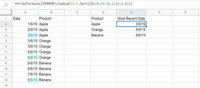
If you know how to use the popular Vlookup function in Docs Sheets, you will definitely find the above formula a lot easier to understand.
VLOOKUP(search_key, range, index, [is_sorted])search_key = D2:D – product names.
range = Sort({B2:B,A2:A},2,0) – The column order changed, I mean moved the product names column from last (second) to first. This is because the Vlookup search key is product names. Sorted the second column, i.e. the date column, in descending order (largest to smallest).
index = 2 – The column index contains the date.
I want to find the 2nd largest date in each group. Then what to do? The above Vlookup won’t work here. I have a new formula for you. See that below.
Array Formula to Find the Nth Largest Date in Each Group in Google Sheets
I have a combination formula that finds the largest dates irrespective of its nth largest element.
That means the formula below is very flexible and can be used to return first, second, or third largest dates in Google Sheets.
It’s a little complex formula. So let me explain to you how to code this formula step by step.
Please enter the below formulas (formulas under step # 1 to 6) in its designated cells. We will combine all these formulas later.
Step # 1 (Cell G2) – Sorting Products and Dates
Sort the range A2:B using the SORT function. It must be like first sorting the product (column 2) in descending order and then by the date (column 1) that also in descending order.
=sort(A2:B,2,0,1,0)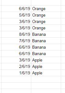
Step # 2 (Cell J2) – Extracting the Second Column
Using the Index function we can return the second column (B2:B) from the above sorted output.
=index(sort(A2:B,2,0,1,0),0,2)Step # 3 (Cell L2) – New Virtual Third Column Containing Running Count
The following formula will count the products and put the sequential number group wise. I mean if product “Apple” repeats twice, it will return the number 1 to the first occurrence and 2 to the second occurrence and so on.
=ARRAYFORMULA(COUNTIFS(B2:B,B2:B,ROW(B2:B),"<="&ROW(B2:B)))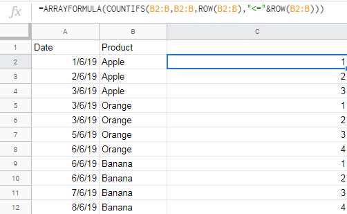
Actually, this is some sort of running count (grouped ranking). I have detailed that here – Running Count in Google Sheets – Formula Examples (please see the comment section in that post for the above formula). You can get the same result using different formulas and the above-linked post contains that. In that, COUNTIFS is the simplest one.
Step # 4 (Cell N2) – Sorted Range in Running Count
In the above COUNTIFS formula replace the range B2:B (with the step # 2 formula as below. You can leave the B2:B within the ROW formula as it is.
=ARRAYFORMULA(COUNTIFS(index(sort(A2:B,2,0,1,0),0,2),index(sort(A2:B,2,0,1,0),0,2),ROW(B2:B),"<="&ROW(B2:B)))Step # 5 (Cell P2)
Combine step # 1 and step # 4 formula to make a 3 column array as below.
Generic Formula:
=ArrayFormula({step#1 formula,step#2 formula})Formula:
=ArrayFormula({sort(A2:B,2,0,1,0),COUNTIFS(index(sort(A2:B,2,0,1,0),0,2),index(sort(A2:B,2,0,1,0),0,2),ROW(A2:A),"<="&ROW(A2:A))})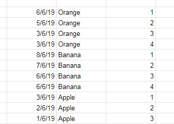
Step # 6 (Cell T2) – Filter the Nth Largest Date in Each Group
Use the above step # 5 data as the data (range) in Query and filter column 3 = nth largest value. Also, you only need to select the columns 2 and 1 only.
=ArrayFormula(Query({sort(A2:B,2,0,1,0),COUNTIFS(index(sort(A2:B,2,0,1,0),0,2),index(sort(A2:B,2,0,1,0),0,2),ROW(A2:A),"<="&ROW(A2:A))},"Select Col2,Col1 where Col3=1"))In this the last part of the code col3=1 controls the nth largest value. 1 means the first largest value, 2 means the second largest value and so on.
Final Step in Cell E2 – Array Formula to Extract the Largest Date in Each Group in Google Sheets
Go to the top of this post. Under the subtitle “Vlookup + Sort combination …” you can find the below formula.
=ArrayFormula(IFERROR(vlookup(D2:D,Sort({B2:B,A2:A},2,0),2,0)))In that replace the code Sort({B2:B,A2:A},2,0) with the formula that I have provided in step # 6 above. You can leave copying the outer ArrayFormula in that formula.
=ArrayFormula(IFERROR(vlookup(D2:D,Query({sort(A2:B,2,0,1,0),COUNTIFS(index(sort(A2:B,2,0,1,0),0,2),index(sort(A2:B,2,0,1,0),0,2),ROW(A2:A),"<="&ROW(A2:A))},"Select Col2,Col1 where Col3=1"),2,0)))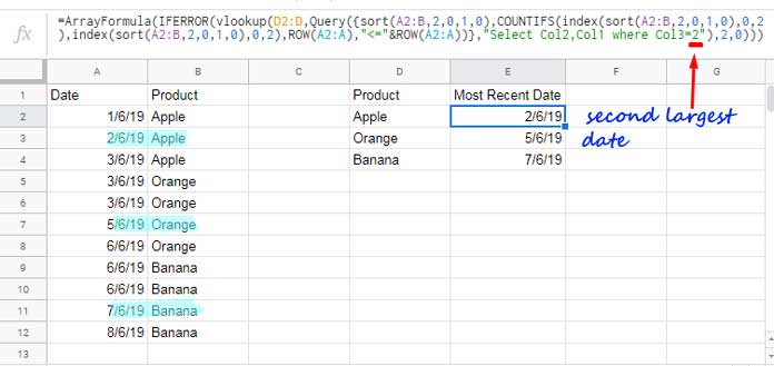
On the screenshot, I have marked the element that controls the nth largest date in the formula. That’s all about extracting the largest date in each group in Google Sheets.
Additional Resources: