


.)
This post explains how to use the LAMBDA function in Google Sheets.
The LAMBDA Function in Google Sheets is simple to learn. We can use it standalone or with a few LHFs (Lambda helper functions). They are MAP, REDUCE, BYROW, BYCOL, SCAN, and MAKEARRAY.
You are well set if you know how to use this function in Excel. As far as I know, the usage is the same in both applications.
In Excel, we use the LAMBDA function with LHFs, and also within “Name Manager” to create easy-to-use custom functions.
Here in Google Sheets also, we use it with LHFs. But it is not a must to create a custom function. The difference lies there.
In this post, let’s learn the LAMBDA function in standalone use. That will help us to grasp the associated helper functions better.
LAMBDA Function Standalone Use in Google Sheets – Syntax and Arguments
Syntax: =LAMBDA([name, ...],formula_expression)(function_call, ...)
Arguments:
1. name – An optional argument called identifier to pass a value(s) to the function. If there are multiple names, put a comma to separate them.
Use it also within the formula_expression and the actual value or cell reference within the function_call. The examples after a few paragraphs below will help you learn this.
Notes:-
- The name(s) must be valid. It must not be cell references like “A1” or “B1.”
- Special characters are not supported except for dots and underscores.
- The name must not start with numbers.
2. formula_expression – The formula that you want to calculate/execute. This argument is required.
3. function_call – Use it to input actual value(s). If no name argument, use () , i.e., open and close brackets.
Note:- When you check the official documentation of the LAMBDA function in Google Sheets, you might find the syntax of it slightly different. I have modified it slightly above to make you understand it clearly.
LAMBDA Function Examples in Google Sheets
The below LAMBDA function examples are to make you understand its usage. At this level, you may even surprise; why this function is even required.
You would only understand the real potential of the LAMBDA function in Google Sheets when you use it together with its helper functions. We will learn that later in my upcoming tutorials.
Examples Leaving the Optional ‘Name’ Argument
As I have said above, the first parameter, i.e., the name, is optional.
In other words, if you don’t want to pass any value to the formula_expression, you can leave it.
Example 1 (Non-Array Formula):
The following Google Sheets CHAR formula will return a heart character in any applied cell.
=char(129505)Output: 🧡
We haven’t used any cell reference in the formula. So, the name argument is not required within the LAMBDA function.
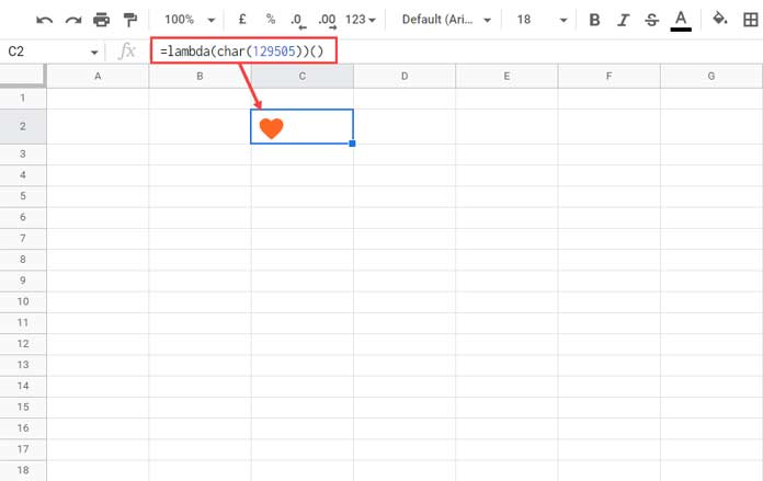
Here is the LAMBDA version of the above CHAR-based formula.
=lambda(char(129505))()In this, char(129505) is the formula_expression. The function_call is the () at the end.
Example 2 (Array Formula):
If B1:B10 is empty, the following formula will return the serial/sequential numbers 1 to 10 in that range.
=arrayformula(row(A1:A10))We can convert this array formula to a LAMBDA formula as follows, where arrayformula(row(A1:A10)) is the formula_expression and () is the function_call.
=lambda(arrayformula(row(A1:A10)))()LAMBDA Function Examples Using All Arguments
To return the love sign (heart symbol) n times, we can use the following formula.
Example 3 (Non-Array Formula):
Enter 5 in cell A1 and the following formula in cell B1 (or any other cell) to return 🧡🧡🧡🧡🧡 characters.
=rept(char(129505),A1)We can convert this REPT-based formula to a LAMBDA one as below.
=lambda(n_times,rept(char(129505),n_times))(A1)Where n_times is the name, rept(char(129505),n_times) is the formula_expression and A1 is the function_call.
Example 4 (Array Formula):
We can flip data in a column or range using the SORT function in Google Sheets.
For example, we have data in A2:B, and we want to flip this data.
Empty C2:D and insert =SORT(A2:B,ROW(A2:A)*N(A2:A<>""),0) in C2 to flip the data.
How to convert this regular formula to a LAMBDA function-based formula in Google Sheets?
We have the formula_expression, which is the above SORT formula.
We can specify the other parameters as follows.
=lambda(
     flip_range,
     first_col_range,
     SORT(flip_range,ROW(first_col_range)*N(first_col_range<>""),0)
)
(A2:B,A2:A)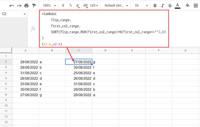
Here we have used two parameters in the name argument. We call it name1 and name2.
name1 – flip_range
name2 – first_col_range
formula_expression – SORT(A2:B,ROW(A2:A)*N(A2:A<>""),0)
function_call – (A2:B,A2:A) where A2:B and A2:A correspond to name1 and name2.
Common Errors
N/A – Wrong number of arguments in use, e.g., the formula doesn’t contain the function_call, a call containing the actual values.
NAME? – When using an invalid identifier in the first argument or a wrong function name used in the formula_expression part.
REF! – Circular dependency.
That’s all about how to use the LAMBDA function in Google Sheets. I’ll explain the other new functions and features based on their availability in the upcoming posts.
Thanks for the stay. Enjoy!