With the help of the UNIQUE and SORTN spreadsheet functions, we can return unique rows in Google Sheets QUERY.

We usually use the UNIQUE function to remove duplicate values. SORTN can also do this, but in a different way, especially with tie mode 2.

The purpose of the Google Sheets QUERY UNIQUE or SORTN combo is to apply the UNIQUE/SORTN function to filtered and summarized (queried) tables.

QUERY is the ultimate solution for creating summary reports and pivot tables. Its aggregation capabilities are exemplary.

In this tutorial, I’ll explain which function to use out of the two (UNIQUE or SORTN) with QUERY to return unique rows with a few examples below.

The syntaxes are as follows:

• UNIQUE + QUERY Syntax: UNIQUE(QUERY())
• SORTN + QUERY Syntax: SORTN(QUERY(),9^99,2,column_index_to_unique,1)

Note: I have omitted the QUERY statements in the above syntaxes because it may vary based on your data and filtering type. You should enter them within quotation marks, as you can see in the examples after a few paragraphs below.

Which syntax should I choose?

Use the UNIQUE formula if your QUERY result has one column. If your QUERY formula result has more than one column, you can use UNIQUE to unique it by all columns, but this may not be what you want.

Use the SORTN formula if your QUERY result has more than one column and you want to unique it by any particular column. SORTN allows you to specify the column you want to unique by, so you can use it to unique your QUERY result by any column.

Return Unique Rows in Google Sheets QUERY: Single Column

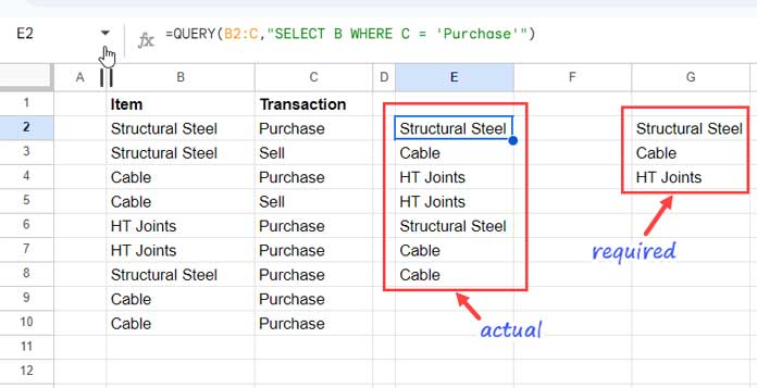
We have a two-column data set, with items in the first column and their transaction type in the second column. We can treat this as a category and subcategory.

The data range is B1:C, where cell range B1:C1 contains the column headers.

I want to filter B2:B if C2:C is “Purchase”, and the following formula does that.

=QUERY(B2:C,"SELECT B WHERE C = 'Purchase'")

Must Read: Learn Google Sheets Query Function: Step-by-Step Guide.

How do we remove duplicate values in the above QUERY result?

We can use the UNIQUE function with it to return unique rows in the above Google Sheets QUERY result.

=UNIQUE(QUERY(B2:C,"SELECT B WHERE C = 'Purchase'"))

This is basic filtering. You can use multiple criteria within QUERY and unique rows as above.

Return Unique Rows in Google Sheets QUERY: Multiple Columns

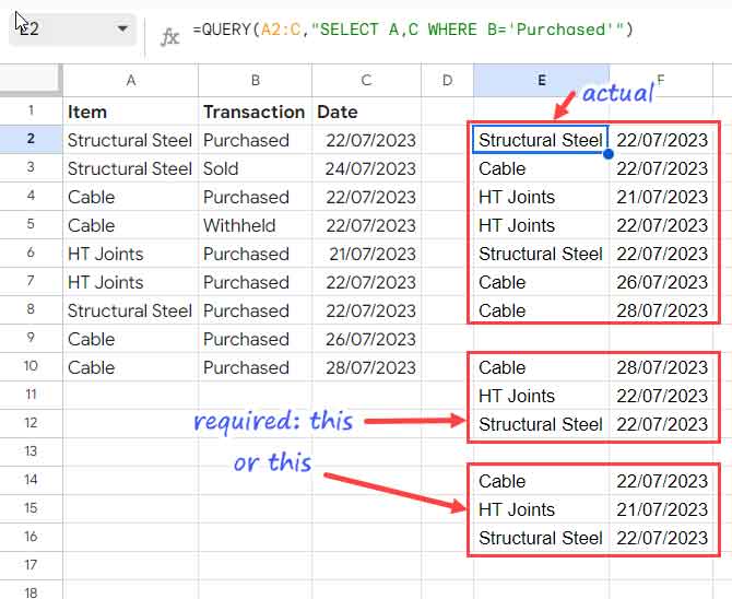
Here is a different dataset with three columns: Item, Transaction, and Date.

The data range is A1:C, where A1:C1 contains the column headers.

I want to filter A2:A and C2:C if B2:B is “Purchased”, and the following formula does that.

=QUERY(A2:C,"SELECT A,C WHERE B='Purchased'")

We cannot use the UNIQUE function to return unique rows in this Google Sheets QUERY result. See my expected results in the above screenshot.

The first result in E10:F12 shows the unique purchased items with the most recent purchase dates, and the second output in E14:F16 shows the oldest purchased items.

We can get the above-expected results in two ways. One is using SORTN, and the other is using QUERY itself. We will see both options below.

Google Sheets QUERY: Unique Rows Using SORTN

To get recently purchased items, you should sort the result in descending order before wrapping the QUERY with SORTN.

Use the ORDER BY clause with QUERY to sort the Date column in descending order. Then wrap SORTN. Here is the formula in cell E10:

=SORTN(QUERY(A2:C,"SELECT A,C WHERE B = 'Purchased' ORDER BY A ASC, C DESC"),9^99,2,1,1)

Note:- Instead of the ORDER BY, you can use the SORT function outside QUERY as a wrapper.

The highlighted index number in the formula represents the unique by column, which is Item.

To get the oldest purchased items, you should sort the result in ascending order before wrapping the QUERY with SORTN.

Use the ORDER BY clause with QUERY to sort the Date column in ascending order. Then wrap SORTN. Here is the formula in cell E14:

=SORTN(QUERY(A2:C,"SELECT A,C WHERE B = 'Purchased' ORDER BY A ASC, C"),9^99,2,1,1)

The above is the SORTN approach to return unique rows in Google Sheets QUERY.

QUERY without Any Wrappers

No doubt, QUERY is the most versatile function in Google Sheets. We can use it without SORTN to get unique rows.

For example, you can replace the formula in cell E10 with this one:

=QUERY(A2:C,"SELECT A,MAX(C) WHERE B = 'Purchased' GROUP BY A LABEL MAX(C)''")

And for cell E14, you can use this one:

=QUERY(A2:C,"SELECT A,MIN(C) WHERE B = 'Purchased' GROUP BY A LABEL MIN(C)''")

You May Like: How to Sum, Avg, Count, Max, and Min in Google Sheets Query.

That’s all about how to return unique rows in Google Sheets QUERY.

Related: How to Find Distinct Rows in Google Sheets Using Query.