Check Time Input in Google Sheets (Formula to Validate Time Cells)

Need to check whether a cell or range contains a time value? In this tutorial, I’ll show you how to check time input in Google Sheets using a formula that works with both single cells and ranges.

Table of Contents

How to Check Time Input in Google Sheets Using TIMEVALUE

Let’s start with a single cell.

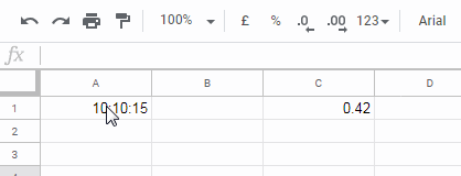
If you use the TIMEVALUE function on a cell like A1, it works only when the cell contains a valid time. Otherwise, it returns an error.

=TIMEVALUE(A1)

Behavior:

If A1 contains only a date, it returns 0.
If A1 contains a valid time, it returns a decimal (e.g., 0.5 for 12:00 PM).
If A1 is empty, or contains text or a number, the formula throws a #VALUE! error.

TIMEVALUE function used to check time input in Google Sheets

To safely detect time, wrap it in an IF formula:

=IF(TIMEVALUE(A1) > 0, TRUE, FALSE)

This returns:

TRUE if it’s a time
FALSE if it’s a date or invalid
#VALUE! if it can’t parse the value

Validate Time Input in a Range

Let’s say you have start and end times in A2 and B2. You want to perform a calculation only if both contain time values:

=B2 - A2

This formula might return incorrect results or errors if either cell doesn’t contain a valid time. Here’s how to check both before calculating:

=ArrayFormula(IF(COUNT(TIMEVALUE(HSTACK(A2, B2))) = 2, B2 - A2, ""))

Explanation:

TIMEVALUE(HSTACK(A2, B2)) checks both cells
COUNT(...) ensures both return valid time values
Only if both are valid, the subtraction happens

If either is not a time, the formula returns a blank ("").

FAQs

Q: How do I check if a cell contains a time in Google Sheets?
A: Use the TIMEVALUE function. If it returns a number greater than 0, the cell contains a time. There is no built-in ISTIME function in Google Sheets.

Q: What happens if the cell contains text or is empty?
A: The TIMEVALUE function will return a #VALUE! error.

Q: Can I check multiple cells at once?
A: Yes. Use ArrayFormula and COUNT(TIMEVALUE(...)) to validate a range.