This is a beginners tips related to Freeze Pane in Google Sheets. Let me explain the use of Freeze Pane with the help of screenshots. Though it’s easy to freeze rows or columns in Google Sheets, you should learn the importance of it. In Google Sheets it’s not only using for freezing rows or columns! You can use Freeze Pane in Google Sheets to set headers in print.
I’ve several medium to advanced level tutorials related to Google Sheets on this page. I realised that I’m lacking some basic tutorials related to it. Earlier, I skipped Google Sheets beginners tips because I thought most of the Google Sheets users were coming from Excel or other similar Spreadsheet applications. But I realised that there are many people who are quite new to spreadsheets. So this tutorial will be useful for such users. So here we begin.
You May Like: Google Sheets Function Guide [Quickly Learn All Popular Functions]
What is Freeze Pane?
Freeze pane is freezing specific number of rows or columns in your spreadsheet. So that it stay there when you scroll the page in any direction. It keeps the sticky behaviour until you remove the Freeze Pane.
How to Set Freeze Pane in Google Sheets
I’m splitting this tutorial related to Freeze Pane in Google Sheets under four sub titles. They are?
- How to Freeze Rows in Google Sheets?
- How to Freeze Columns in Google Sheets?
- Freeze Rows and Columns Together in Google Sheets.
- Freeze Pane to Set as Headers or Page Titles in Google Sheets.
How to Freeze Rows in Google Sheets
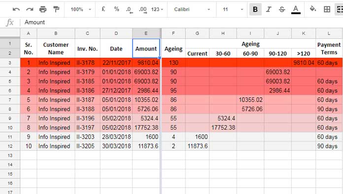
To demonstrate, I am going to use one of my custom heat map file. See the screenshot. In this certain cells in the first two rows are merged. It’s the titles of my heat map.

To freeze these two rows, I mean to make it say there when I scroll to down the page, just follow the below steps.
Click the very first cell in the third row. Here it’s cell A3. Then as seen on the screenshot go to the menu View > Freeze > 2 rows.
Also Google Sheet can show you the number of rows to freeze based on your current position (active cell) in the sheet. If you are on row # 6, if you access the View menu Freeze, you can see the suggestion “up to current row (6)”. But it won’t work if your cells are merged.
How to Freeze Columns in Google Sheets
Freeze Pane in Google Sheets can also freeze columns. But it’s not common in use. Users either freeze rows or freeze rows and columns together. But we can freeze columns only.
Please make sure that you are in the very first row on your sheet. For example I want to freeze up to column E. See the below image. To do that click on cell E1 and go to the View menu Freeze Pane and click on “Up to current column (E)”. That dark shaded line is the Freeze pane identification on a sheet.

How to Freeze Rows and Columns Together in Google Sheets
With one click you can’t freeze columns and rows together. First freeze rows and then freeze columns as said above.

You may be interested in knowing what I did in the above freezing of rows and columns. So here is the steps.
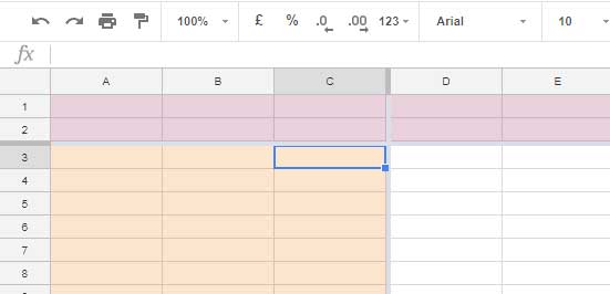
My active cell is C3. I did the settings as below.
View > Freeze > Up to current column (C)
View > Freeze > 2 rows.
How to Unfreeze Columns / Rows in Google Sheets?
You can unfreeze rows and columns from the above same View menu Freeze.
The Role of Freeze Pane in Google Sheets Header
If you have lots of rows in your Google spreadsheet, when you print it may spread across several sheets. So you may want the first row or first few rows repeated in every page as title rows. Possibly your first row may contain the column headers / titles. In such cases you can use this freeze pane feature in Google Sheets. Just freeze the rows that you want to print as titles. It acts as header or you can say print titles. Please refer my below post for detailed info on printing titles / headings in Google Sheets.
Must Read: Repeat Page Titles in Google Sheets
That’s all about Freeze Pane in Google Sheets. Enjoy!


