This tutorial explains how to repeat page titles at the top or left of pages in printouts using frozen rows and columns in Google Sheets.

Repeating page titles on every page is important when printing your data because it makes your printout reader-friendly.

To repeat page titles, add the header row (the top row with labels) to the top of every printed page or add the first column (the left column with labels) to the left of every printed page.

If you do not use the print title feature in Google Sheets, you can manually copy and paste the title row to the top of each page or the first column to the left of each page. However, this will destroy your data structure and affect filtering and formulas in the sheet.

Therefore, it is best to use the print title feature whenever you need to print multiple pages of spreadsheet data in Google Sheets.

How to Print Page Titles on Every Page in Google Sheets

Google Sheets does not allow you to select a row or column from the middle of a table and repeat it as the page title on every page. Instead, Google Sheets can only print titles up to the header row or column, because it uses the Freeze rows and columns feature for this.

The Freeze feature allows you to lock your rows, columns, or both in a Sheet. Let’s see how it affects printing in Google Sheets.

Repeat Page Titles at the Top of Printed Pages

To repeat page titles on the top of every printed page in Google Sheets, follow these steps:

Remove any frozen rows and columns. To do this, click View > Freeze > No rows and then View > Freeze > No columns.

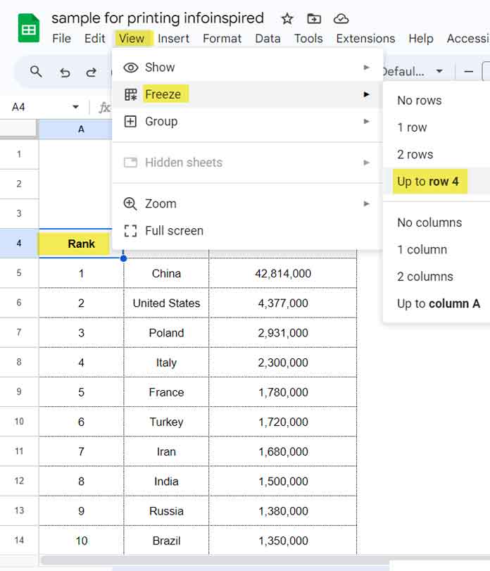
Go to the row that you want to repeat at the top of every printed page. In our example, this is row 4.

Click View > Freeze > Up to row 4. This will place a shaded bar at the bottom of row 4 across the row. Hereafter, when you scroll the page down, the top four rows will be frozen.

Click File > Print. This will open the print dialog box (a sidebar panel) on the right-hand side of the screen.

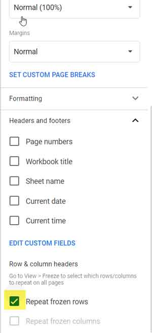
Scroll down to the bottom of the print dialog box and make sure that “Repeat frozen rows” under the “Row & Column headers” is checked. If not, check it.

Click Next (a blue button at the top) > Print.

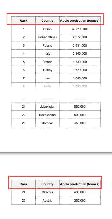
When you print your Google Sheets data, you will see the page titles repeated on each and every page.

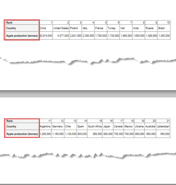
Repeat Page Titles at the Left of Printed Pages

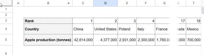
In the above example, we have vertically arranged data, so we have a header row to repeat on every printed page. But what about horizontally arranged data?

Assume we have transposed the above same sample data. Then we have columns to repeat on every page, not rows.

To repeat page titles in columns on every page, follow these steps:

1. Remove any frozen rows and columns (View > Freeze > No rows/No columns).
2. Go to the column that you want to repeat at the top of every printed page. In our example, this is column B.
3. Click View > Freeze > Up to column B. This will place a shaded bar at the right-hand side of column B down the column. Hereafter, when you scroll the page to the right-hand side, the left two columns will be frozen.
4. Click File > Print.
5. On the print dialog box, make sure that “Repeat frozen columns” is checked. If not, check it.
6. See the preview.

Conclusion

Do you see any drawbacks to the current repeat rows settings using frozen rows and columns in Google Sheets?

Yes, there is one drawback. When you repeat print titles on the top of a spreadsheet, any values in the frozen rows will be repeated on the top of every page. This can be a problem if you have important data in the frozen rows that you don’t want to be repeated.

For example, if you have frozen the top 4 rows of a spreadsheet, but the header row is in row 4, then any values in rows 1 to 3 will be repeated on the top of every page.

Keep this in mind when using the repeat rows or columns settings in Google Sheets when printing.