To filter unique digit numbers in Google Sheets, first you need to know how to test whether a provided number contains unique digits. This is applicable to highlighting (conditional formatting) also.
A unique digit number means a number with unique digits. For example 98765 is a distinct/unique digit number (it is the largest unique 5 digit number also).
Another example is 10234 (which is the smallest unique 5 digit number).
We are not talking about the largest or smallest unique n digit numbers. Our topic is unique/distinct digit numbers.
It can be the smallest, largest, or can contain any number of digits but the digits in the number must be unique or not repeated.
In this post we can learn how to filter the unique digit numbers from a list of numbers in Google Sheets.
How to Filter Unique Digit Numbers in Google Sheets
There are 4 steps involved. They are extracting the digits, unique it and count, match the count with the length of the number in question and filter.
Extracts Digits from a Number to a Column
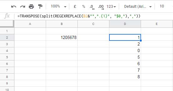
As said above, to test whether all the digits in a number is unique, we need to extract all the digits first. We can use the following formula for that (extracting digits).
If the number is in cell B2, then we can use the below REGEXREPLACE, SPLIT, and TRANSPOSE combination formula (always read the combination formula from the middle).
=TRANSPOSE(split(REGEXREPLACE(B2&"",".{1}", "$0,"),","))There are two more formulas that we can use for the same purpose. You can get those formulas here – Split a Number to Digits in Google Sheets. But I’m comfortable with the above combo.

Formula Explanation
The key is the REGEXREPLACE which inserts (puts) a comma after each digit.
=REGEXREPLACE(B2&"",".{1}", "$0,")Result: 1,2,0,5,6,7,8,
Syntax: REGEXREPLACE(text, regular_expression, replacement)The .{1} part of the REGEXREPLACE formula (regular_expression) matches any character (except for line terminators) one time.
Yes! it matches ‘characters’. That is why I’ve formatted the number in cell B2 to text by joining a null character to it, i.e. B2&"".
The $0, part of the REGEXREPLACE formula (replacement), inserts a comma after each digit.
Note: If you use (.{1}) as the regular_expression, then the replacement must be "$1,. It’s equal to the above.
The SPLIT splits the digits as the delimiter to split is the ",".
The split digits will be in a row. The Transpose function helps to change the orientation to a column so that we can use this within Unique.
Unique and Count the Extracted Digits
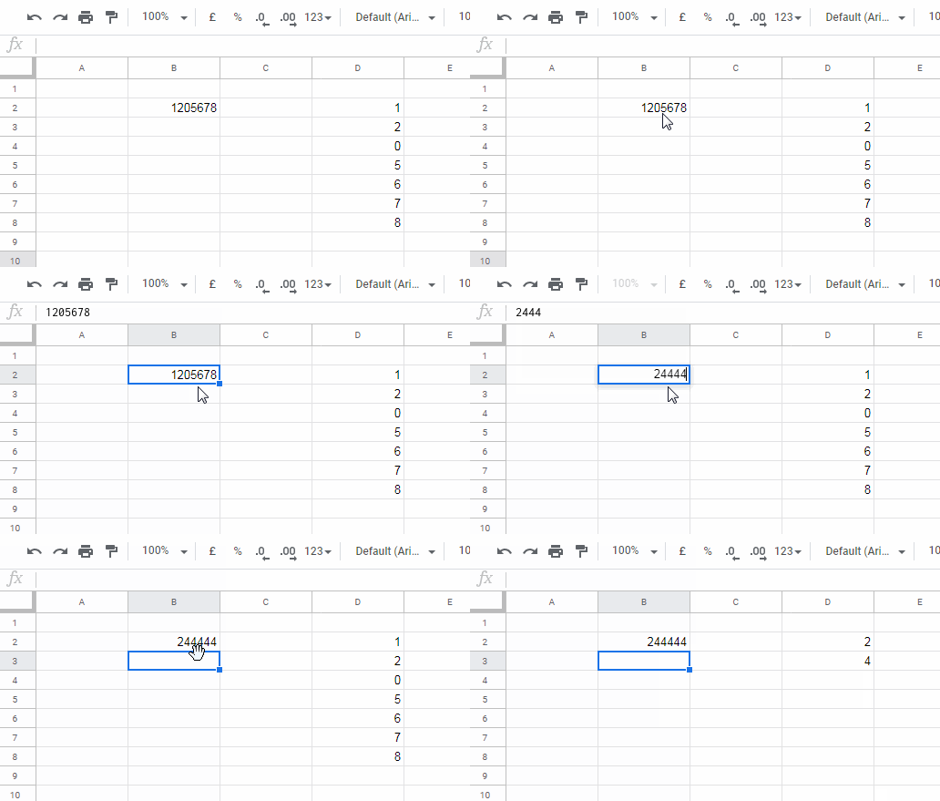
Let’s unique the returned digits by wrapping the formula with Unique. The below formula (unique_digits_formula) removes any repeated digits from the extracted digits.
=unique(TRANSPOSE(split(REGEXREPLACE(B2&"",".{1}", "$0,"),",")))
Test Whether the Provided Number Is a Unique Digit Number in Google Sheets
Now to test whether the provided number is a unique digit number in Google Sheets, just check whether the count of the digits in the above formula output matches the length of the number in cell B2.
We can get the length of the number in cell B2 by using the LEN as below.
=len(B2)To get the count of the unique digits wrap our earlier formula with COUNTA (you can use COUNT also). That means in generic form;
=counta(unique_digits_formula)=len(B2)Here is the formula to test whether the provided number is a unique digit number in Google Sheets.
=counta(unique(TRANSPOSE(split(REGEXREPLACE(B2&"",".{1}", "$0,"),","))))=len(B2)The above formula would return FALSE if the number is not a unique digit number, else TRUE.
Filter (Helper Column Involved)
When there is a list of numbers in a column in Google Sheets, and you want to filter only the unique digit numbers from it, use the below method.
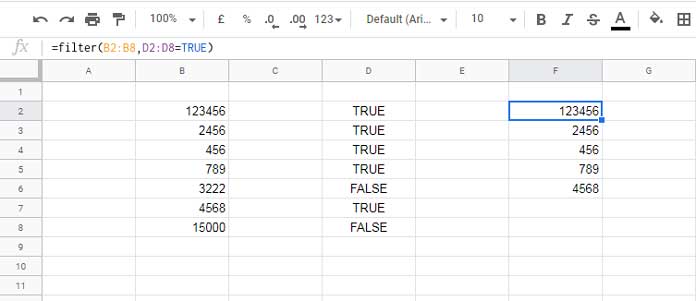
The list as per my example is in cell B2:B8. My above formula is in cell D2. Drag the D2 formula to D8. Then use the below Filter formula in cell F2.
=filter(B2:B8,D2:D8=TRUE)
The Filter filters B2:B8 if column D2:D8 is TRUE.
Filter (Without Helper Column) Unique Digit Numbers by Cell by Color
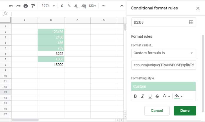
This is an additional tip. instead of filtering, if you want to highlight the unique digit numbers in a sheet, we can use the below formula rule.
- Select the range, here B2:B8.
- Click Format > Conditional Formatting > Format Rules > Custom Formula is;
In the given blank field, copy paste the following formula.
=counta(unique(TRANSPOSE(split(REGEXREPLACE(B2&"",".{1}", "$0,"),","))))=len(B2)This is the formula that you can find just above the sub-title ‘Filter (Helper Column Involved)‘.

Now you may be able to filter the highlighted color using the Filter by Color feature (Data > Create a filter > Filter by color).
How to Highlight Only N Distinct Digit Numbers in Google Sheets
I want to only highlight those numbers that have 5 digits and the digits are unique. Then what to do?
If this is your question, the answer is simple. Just use the AND logical operator with the above formula to test whether the number has 5 digits other than unique.
=and(counta(unique(TRANSPOSE(split(REGEXREPLACE(B2&"",".{1}", "$0,"),","))))=len(B2),len(B2)=5)In this len(B2)=5 controls the ‘n’.
That’s all. Enjoy!


