Extracting the first letter of each word in a string is easy in Google Sheets. The real challenge is transforming it into an array formula.
To extract the first letter of each word, we will first split the string and then use the REGEXEXTRACT or LEFT function to extract the first character.
Let’s assume cell A3 contains the string “North Atlantic Treaty Organization”.
I want to extract the letters “N”, “A”, “T”, and “O”, and later join them as an abbreviation like “NATO”. Here is how we do that in Google Sheets.
Formulas to Extract First Letters from Each Word in Google Sheets
Using SPLIT and LEFT Combo:
=ArrayFormula(LEFT(SPLIT(A3, " "), 1))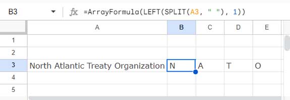
Here, the SPLIT function splits the string at each space character, and the LEFT function extracts 1 character from the left of each split word.
Using SPLIT and REGEXEXTRACT Combo:
=ArrayFormula(REGEXEXTRACT(SPLIT(A3, " ")&"", "."))In this case, the SPLIT function splits the string. We added "" to the split words to ensure they are treated as text, a precaution to avoid errors in case any split part is numeric. Then the REGEXEXTRACT function extracts one character from each word.
Both of these formulas use the ARRAYFORMULA function since they return array results.
Can These Formulas Be Used in a Range?
You can use both formulas in a range like A3:A. However, remember to include the IFERROR wrapper; otherwise, you will see error values in rows where A3:A is blank.
Here are the array formulas to extract the first letter of each word in a string in Google Sheets:
=ArrayFormula(IFERROR(LEFT(SPLIT(A3:A, " "), 1)))
=ArrayFormula(IFERROR(REGEXEXTRACT(SPLIT(A3:A, " ")&"", ".")))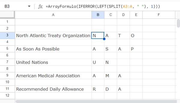
If you don’t use the IFERROR wrapper, the first formula will return #VALUE! errors in blank rows. The second formula will return #VALUE! errors in blank rows and #N/A errors in empty columns as well.
Extracting and Joining the First Letter of Each Word to Form an Abbreviation
When you extract the first characters from a cell, not a range, you can combine the characters extracted to form an abbreviation using the JOIN function as follows:
=JOIN("", ArrayFormula(LEFT(SPLIT(A3, " "), 1)))
=JOIN("", ArrayFormula(REGEXEXTRACT(SPLIT(A3, " ")&"", ".")))
This will return ‘NATO’ instead of ‘N’, ‘A’, ‘T’, and ‘O’ individually.
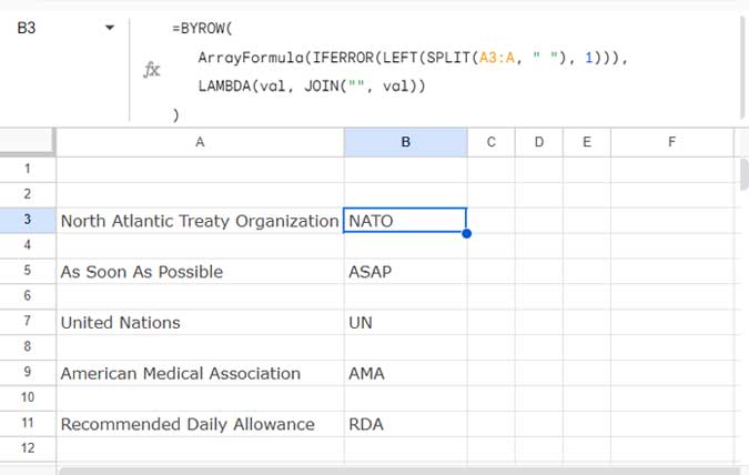
If you want to auto-extend the formula down the column, you can use the BYROW function as follows:
=BYROW(
   ArrayFormula(IFERROR(LEFT(SPLIT(A3:A, " "), 1))),
   LAMBDA(val, JOIN("", val))
)
You can replace ArrayFormula(IFERROR(LEFT(SPLIT(A3:A, " "), 1))) with ArrayFormula(IFERROR(REGEXEXTRACT(SPLIT(A3:A, " ")&"", "."))) as well.
If you want the joined text separated by a space, replace the delimiter in the JOIN function, i.e., "" with " ". So the formula will be:
=BYROW(ArrayFormula(IFERROR(LEFT(SPLIT(A3:A, " "), 1))), LAMBDA(val, JOIN(" ", val)))Note: The BYROW function is resource-intensive, and you may encounter performance issues when applying it to a very large dataset.
You can skip the following section as it just details the functionality of the above formula.
Formula Explanation
The BYROW function applies a lambda function to each row in an array and groups each row into a single value. The result will be a new column.
Syntax:
BYROW(array_or_range, lambda)array_or_range:ArrayFormula(IFERROR(LEFT(SPLIT(A3:A, " "), 1)))(one of the formulas that splits strings and extracts the first letter of each word).lambda:LAMBDA(val, JOIN("", val))(The JOIN function that concatenates each element in the array, defined as ‘val’, using the""delimiter).
This returns a new column array formed by grouping each row in array_or_range into a single concatenated value. The grouped value for a row is obtained by applying a lambda on that row.


