


")

")


We can create a multi-row dynamic dependent drop-down list in Google Sheets without using Google Apps Script. This tutorial explains how.
I will only use built-in Google Sheets functions to create a multi-row dynamic dependent drop-down list.
Why Are Dynamic Dependent Drop-Down Lists Useful?
Let me explain why a dynamic dependent drop-down list in Google Sheets is a must-try.
Imagine you are running a bookstore. You can create two drop-down lists: one containing all the author names and the other their book titles, and copy them in multiple rows.
When you receive inquiries, for example, from educational institutions, you can share the sheet with them.
They can select the authors and book titles from the drop-downs.
There are plenty of such situations where you can use dynamic dependent drop-down lists.
Creating a Simple Drop-Down List in Google Sheets
Anyone with limited spreadsheet experience can easily create a simple drop-down list, not dynamic. How?
I must explain this part before starting the tutorial on creating a dynamic dependent drop-down list because it is the essence of the tutorial.
Your first drop-down menu in Google Sheets is just a click away. To create a simple drop-down list, please follow these steps:
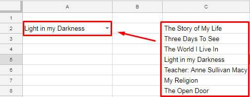
I have the list of items to include in the drop-down list in C2:C8 (Sheet2). I’m going to create the drop-down in the same sheet, cell A2.
Steps:
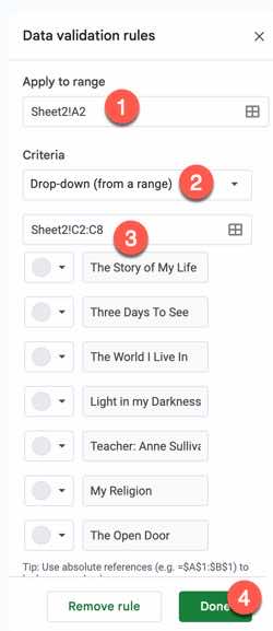
- Navigate to cell A2 in “Sheet2”.
- Go to the menu Insert > Drop-down.
- Under Criteria, select Drop-down (from a range).
- Enter the range
Sheet2!C2:C8in the given field. - Click Done.
Please refer to the screenshot below.
It’s that simple.
Now let us move to more complex forms of the drop-down list.
How to Create a Dependent Drop-Down List in Google Sheets
To create a dependent drop-down, you first need a basic drop-down list. It works like this:
You select the author name “Leo Tolstoy” in cell A2. Then, all of this legendary author’s books will be available to pick from the drop-down in cell B2.
When you pick another author from the list, the list of books in cell B2 should change accordingly.
The dependent drop-down list is also called a Dynamic Dependent Drop-down List because the values in it change based on the value selected in its parent.
Now, let us learn how to create a dependent drop-down list in Google Sheets.
Sample Data:
| Agatha Christie | Sir Arthur Conan Doyle | Helen Keller | Leo Tolstoy |
| The Mysterious Affair at Styles | The Adventures of Sherlock Holmes | The Story of My Life | Anna Karenina |
| The Murder on the Links | A Study in Scarlet | Three Days to See | The Kreutzer Sonata |
| The Big Four | The Return of Sherlock Holmes | Light in My Darkness | Sevastopol Sketches |
| The Mystery of the Blue Train | His Last Bow | Teacher: Anne Sullivan Macy | Resurrection |
I have the above sample data in the cell range A1:D in Sheet2 where A1:D1 contains author names (which we will use for creating the drop-down list in A2 in Sheet1) and the cell range A2:D contains books of the respective authors (which we will use to create the dynamic dependent drop-down list in B2 in Sheet1).
Step 1: Creating the Parent Drop-Down
Here we will use the names of authors for the parent drop-down list.
- Navigate to cell A2 in “Sheet1”.
- Go to the menu Insert > Drop-down.
- Under Criteria, select Drop-down (from a range).
- Enter the range
Sheet2!A1:D1in the given field. - Click Done.
Step 2: Formula Part
Navigate to cell E2 in Sheet2 and enter the following XLOOKUP formula:
=TOROW(XLOOKUP(Sheet1!A2, A1:D1, A2:D, ), 1)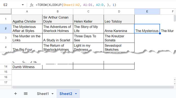
This XLOOKUP formula searches for the author name selected in Sheet1!A2 within the range Sheet2!A1:D1 and returns the corresponding books from Sheet2!A2:D.
The TOROW function converts values from a column into a row and removes empty cells from the result.
This formula dynamically connects the selected author in the parent drop-down to their corresponding book titles.
Step 3: Creating the Dynamic Dependent Drop-Down List
Now we can move to the final step, i.e., creating the dependent drop-down list.
- Navigate to cell B2 in “Sheet1”.
- Go to the menu Insert > Drop-down.
- Under Criteria, select Drop-down (from a range).
- Enter the range
Sheet2!E2:2in the given field. - Click Done.
Your dependent drop-down list is ready. Select any author in cell A2, and the corresponding books will be available for selection in cell B2.
How to Create a Multi-Row Dynamic Dependent Drop-Down List in Google Sheets
Now let us create a multi-row dynamic dependent drop-down list.
You need to adjust two settings: one is to modify the formula in cell E2 in Sheet2, and the other is in the dependent drop-down in cell B2 in Sheet1.
Let’s first edit the dependent drop-down.
- Navigate to Sheet1!B2.
- Click Insert > Drop-down.
- Under Criteria, you will see the range as
=Sheet2!$E$2:$2. It’s an absolute reference always pointing to the range E2:2 in Sheet2. To make it relative, remove the dollar sign. Edit it to look like this:=Sheet2!E2:2.
Then select cells A2:B2 (the parent and dependent drop-downs) and drag the fill handle down as far as you want.
In Sheet2!E2, replace the earlier formula with the following one, which will expand the XLOOKUP down:
=MAP(Sheet1!A2:A, LAMBDA(r, TOROW(XLOOKUP(r, A1:D1, A2:D,), 1)))Where:
Sheet1!A2:Ais the parent drop-down range in Sheet1.A1:D1contains the author names used for the parent drop-down.A2:Dcontains the book titles used for the dependent drop-down.
Your dynamic-dependent drop-down list is ready.
This formula uses the MAP and LAMBDA functions to expand the XLOOKUP results down based on the author names selected in Sheet1!A2:A. Please note that LAMBDA functions can consume more resources.
Resources
- Create Multiple-Selection Dependent Drop-Downs in Google Sheets (New!)
- Auto-Populate Information Based on Drop-Down Selection in Google Sheets
- Display Data from Any Sheet with Google Sheets Drop-Downs
- Distinct Values in Drop-Down List in Google Sheets
- Getting an All Selection Option in a Drop-Down in Google Sheets
- Populate an Entire Month’s Dates Based on a Drop-Down in Google Sheets
- Create a Drop-Down to Filter Data From Rows and Columns
- Create a Drop-Down Menu From Multiple Ranges in Google Sheets
- How to Combine Multiple Sheets in Importrange and Control Via Drop-Down
- Relative Reference in Drop-Down Menu in Google Sheets
Hello,
I have successfully used the BYROW formula. However, I wish to create a filter, so I can use sort A-Z.
When I attempt this, my cells containing dropdown lists return an error message that reads, “Input must fall within the specified range.” Any tips on how to fix this? Thank you!
Hi, LG,
Sorry! I’m unable to answer without seeing a sample of your data.
Here is the link to my copy of your sample sheet spreadsheet:
— URL remove by admin.
Hi, LG,
Thanks for sharing a sample copy. I tested and found sorting re-arrange the drop-downs as per the value in another column. But the range inside drop-downs doesn’t move because of the array formula. Sorry, I don’t find a workaround.
Hey and TY!
I believe it’s a good idea to create lists by pivoting any other list of data Author Book. I mean Sheet1 C:F columns.
We can’t pivot without aggregation but it feels like we can pivot by
=TRANSPOSE(UNIQUE...for the 1-st row and=BYCOL(***lambda(***FILTER(...for all other rows.Hi, Max,
I am afraid you missed my BYROW formula in this tutorial.
Hi Prashanth,
How do you use “Any” as a selection in a Dynamic dropdown box to display all data? I have tried “Any,” and
*.*neither works.Hi, Ron,
You may check this – Getting an All Selection Option in a Drop-down in Google Sheets.
Hi! I am also trying to add more “author names” (in my case, car make and model) to my sheets, but I am unable to do so.
– URL removed by Admin –
Could you kindly help advise how I can do it by changing your suggested formula? Thanks for sharing.
Hi, Esther Ng,
Insert this new formula in cell G1. I’ve updated my tutorial and also my sample Sheet.
=byrow(A1:A,lambda(r,ifna(transpose(filter(C2:H,C1:H1=r)))))This formula doesn’t require Named Ranges.
Hi Prashanth,
Can you help me with having the dynamic dependent drop-down on the same column, i.e., A2 (author name) -> A3 (books), B2 (author name) -> B3 (books), and so on?
I read in the older comments that it wasn’t solved with this method.
Did you find a way to achieve this, or can you maybe, redirect me to a helpful formula/blog/script?
Hi, Varun,
I’ve added a new tab named “Sheet2” in my sample Sheet, where you can find the solution to your problem.
Hey,
Everything works well, but on my side, when I insert a new row (for example, above row 10) (it’s a use case that I can have in my google shared document with my team), I lose the right dependent lists in this new row and all the row below.
The data validation in the new row and the row below is offset.
How can I solve this issue?
Hi, Jérémy,
I couldn’t replicate the problem on my side.
Consider sharing a copy (filled with mockup data).
You can include the URL in your reply below.
Hi Prashanth,
Thank you so much for this. However, I need one help.
Look into the file. I did everything you showed for this to work.
The F2 (Sub Category) returns the correct value for E2 (Root Cause). But how do I apply the same thing to the entire sheet?
— URL removed by admin —
Hi, Raaj Pathak,
The formula should be in the last column so that it can expand.
I’ve updated your Sheet with the correct formula and its placement.
Hello!
I have multiple “author names” in my worksheet, so I have replicated
if(transpose(A1:A)=D1,indirect("Sir_Arthur_Conan_Doyle")for each “author” I have.However, it gives me the correct results only for the first 4 “authors”. How do I get the data for the remaining ones?
Not sure if this has something to do with the IF formula limitation?
Thanks!
Hi, Preksha,
I am happy to help if you can share a copy of that sheet. You can leave the URL in your comment reply.
Hi Prashanth,
Thanks! I’ve left the URL and my notes.
Hope that helps!
Hi, Preksha,
Your last part of the formula is
INDIRECT("")))))),"")))))))which is wrong. It should beINDIRECT("Freelancers"))))))))))),""))I’ve already modified your Sheet.
Can you please share me the Apps Script?
Hi, Vivek Shah,
Please check ‘older comments’.
Thank you so much. This is exactly what I needed! You explained it so well!
Hi Prashanth,
I have a problem using the formula you posted for cell E2.
=if(A2=C2,indirect("Helen_Keller"),Indirect("Leo_Tolstoy"))I always get a parse error.
Can you please help me?
=if(A2=C2,indirect("apple"),Indirect("plum"))Hi, Paul,
Please make sure that you have created the named ranges.
Also, the parse error might be due to the LOCALE settings.
You can share an example sheet for me to check by leaving the URL in the ‘reply’ below.
I have a question to ask. I select a value in the drop-down (say column B2), I need to populate a matching value in C2 based on the value in B2.
May be B column contains vendor and c column telephone#
How can this be done? Can you help?
Hi, ananda,
We may be able to use Vlookup. You can leave a sample Sheet’s URL below.
I’m having issues retaining the formula in the first cell of the row so that it isn’t broken by a sort.
I think the fix is to have arrayformula in the header, but I’m not sure how to retain functionality by either including a title or having the functionality start on the next row.
Hi,
Please try this fix – How to Stop Array Formula Messing up in Sorting in Google Sheets.
Thanks for this, this is great.
One thing I’m running into issues with is if I sort the column B (it is a date in my case), the reference between the two columns is broken to different rows. Instead of A1 corresponding with B1, A1 corresponds with B3 or something after the sort. I have quite a bit of drop downs, so everything is on a different sheet. Any thoughts on how to fix that?
Thank you!
Your chain of “if” statements seems like it could get clunky if you have hundreds of authors you could look up.
One edit that I made to your method was to avoid having to do all those “if” statements in your array formula.
I just did;
=arrayformula(transpose(indirect(substitute(A2, " ", "_"))))The upside is that it automatically pulls the correct named range without the “if” statements.
It does have the downside that I couldn’t get the arrayformula doesn’t fill down all the way anymore.
So you have to drag and copy it down. And you’d still have to create all those named ranges.
Hi, Eugene,
I agree with you, and thanks for your feedback.
That is so helpful!
I don’t need one Array Formula. I used automatic filling so that some hidden columns always show a single array formula dependent on the adjacent cell in the row.
This formula is much simpler.
Thank you also, Prashanth, for your help, great as always!
Can you explain this, please? I am trying to understand how to do it for my finance tracker.
Hi, Andrea,
He seems to use the ‘Auto Fill’ suggestion to fill column G, instead of using an auto-expanding array formula in cell G1.
Hi,
It is the best help I have found so far. But I’m having problems when adding columns in between.
I see your sample in the tutorial having no problems with it, but mine won’t have the correct dependent dropdown and array of options.
Did you still use the script for this? I hope you can help me soon. Thanks!
Here’s an editable copy for your reference.
— link removed by admin —
Hi, Celestina,
Nope! I have not used any Apps Script.
In my example sheet, I have used an array formula in Sheet1!G1.
In the place of that, you have used a non-array (drag-down) formula in MAIN!D3, which I have modified.
In addition to that, I have modified your named rages. You were using a whole column range, which may cause issues. I have used a small limited range instead.
Please, check your sheet.
Oh, I see the difference.
I guess I didn’t exactly copy and modified the formula correctly.
May I ask, how exactly did I make it a non-array formula? Is it because I put (A3) instead of (A:A3)?
Also, I made the ranges with 20 columns only. The whole column range did cause some errors.
Hi, Celestina,
You can find two formulas below the sub-title “Now the Formula Part in Multi-Row Dynamic Dependent Drop Down List In Google Sheets.”
To know the array/non-array difference, please compare them.
How can I add extra columns with more data?
When I try to extend out your formula I start getting “Array arguments to IF are of different size.” errors
I am receiving the same issue, otherwise working perfectly. Any solutions?
Hey, I am currently using a separate tab to keep my transposed rows. I need to be able to delete, move, filter, and insert rows into my original sheet (with the dropdowns). Is this possible? Currently, it causes errors. Any help appreciated.
Hello,
What can I do if I want to have in column A a “company list” and in column B “the list of contact”s who are attached to the company?
Knowing that new contacts can be attached to each company.
Thx
Hi, laurent,
Replace C1:F1 with company names (this will create the company list). In my example, this cell range contains author names.
Replace C2:F with corresponding contacts. In my example, this cell range contains book titles.
Thank you so much.
Thanks, Prashanth for the update. Will look forward to the new feature reflecting soon.
Regards,
Sunil
Hi. Sorry to interrupt you. Would you please explain the following two things to me?
len(A1:A),transpose(A1:A)=C1What does A1:A mean?
Hi, Martin,
A1:A is column A which contains the drop-downs.
len(A1:A)means non-blank cells in the range A1:A.The function TRANSPOSE used to change the column orientation (vertical to horizontal).
The question here – If I add a new row to the sheet, here my formulae is going for a toss – how to avoid that?
Hi, Jaishree,
I couldn’t reproduce that issue in the example sheet that I included within this tutorial.
Hello Prashant,
I tried everything as you mentioned post the update but when it comes to mentioning
='Sheet1'!$H$16:$K$16in the Data range under Data validation (C1:F1 as per your example), when I click save, there is a red error box appears and it says “Please enter a valid range”.Could you please help here because only the first cell works (A1 for you and D3 for me) but when I copy and paste further below, nothing shows up in (B2, your example)?
Could you please help?
Thanks,
Sunil
In your example of B1 > Data > Data Validation > enter data range > here the system is not accepting when I type
='Sheet1'!G1:T1. It says “Please enter a valid range”.Please help.
Thanks,
Sunil
Hi, Sunil,
Please make sure you spelled the sheet name correctly.
Also, you can check my example sheet for the same.
Hi Prashant,
Yes, I’ve spelled it correctly, and also checked your example sheet, which very clearly has the data range starting from = and also accepts the $ value prefixed to the cells. When I do the same, the error message is “Please enter a valid range”.
I’ve spent hours just re-entering the data validation range in multiple options, but it never worked.
Please do help me.
Thanks,
Sunil
Hi, Sunil,
It’s actually a new Google Sheets feature. I think it’s not yet rolled out fully. So please wait a few more days.
Hi,
I have managed to do all the formulas. My only problem is copying B1 downwards. The list range does not automatically copy. I have about 1000 rows.
Hi, Rachel,
Earlier there was the issue. Now the drop-down supports relative reference.
In B1, the data validation “List from a range” must be
=G1:T1, not=$G$1:$T$1.When you copy down you will see the copied drop-down flagged. Just delete the values by selecting B2:B1000.
Related – Relative Reference in Drop-Down Menu in Google Sheets.
Hello Prashanth,
Following is the link to the sheet.
… link copied and then removed by the admin …
Would like your help in resolving this issue I’m facing.
I have managed to get data validated in the same row depending on the selection of cell A1. But I would like to get it vertically.
Eg.: Cell B2 has (rooms)
Need B3 to give dynamic data validation depending on the room type selected in B2.
Hi, Raju,
I have gone through your sheet to understand your requirement. You want the drop-down and the dependent drop-down in the same column.
My solution won’t be able to fulfill your requirement as the formula in G1 populates the dependent drop-down values (B1:B drop-down) based on the values in column A (A1:A drop-down).
When I drag the validation column to below, dependent data validation not dynamically changed. There is needed one by one data validation.
I need an entire column, could you please help me.
Hi, OM Kumar Chaurasiya,
You may require to use Apps Script. Please go thru’ the comments to find the relevant link.
Hi, OM Kumar Chaurasiya,
It changes now. Thanks, Google for the update.
You may please check my tutorial once again to see the update.
Hi Prashanth,
I have used your formula for 10 column data. I have added values accordingly but the formula works only for 4 columns.
I’m getting the error “Wrong number of arguments to IF. Expected between 2 and 3 arguments, but received 4 arguments.”
Can you help?
Sheet URL (with edit access) please.
Thanks for this! The only issue I’m currently having is that I get #N/As appearing in my dropdown list because the lists are shorter. Is there a way to avoid this? Thanks in advance.
Use IFNA() to remove the N/A errors from the data validation range. I haven’t seen that issue in my test.
Thanks for this! It was quite helpful, and while a little clunky, it allowed me to do exactly what I needed to do. Nevermind manually changing 200 cells…it is still much better than the alternatives.
Hi, Onyx,
Now, no need to manually change the rows. I have updated the tutorial based on the lastest Google Sheets program changes.
How can I add a third column? A dependent list for the first dependent list?
Thank you so much, I used your example and was able to create a basic work order for our flooring business. One question that I have, how can I now connect the options to a price in a third column? For example Author > Title > Price. I would love to do that but my understanding of sheets and excel is limited.
Hi, Kelly,
You can maintain a price list in another tab and use Vlookup. If you can share a copy (just demo data) of your Sheet, I may be able to help you.
Best,
My multiple dropdowns work, as long as I do not sort. If I want to sort alphabetically then the data validation gets messed up. Suggestions?
Hi,
Open a new tab and use the SORT formula.
=sort(Sheet1!A1:B,1,true,2,true)If you want you can filter the author too.
=filter(Sheet1!A1:B,Sheet1!A1:A="Helen Keller")Best,
Prashanth KV
“This’s because while copy and pastes a data validation list, there is no option in Google Sheets to change the range automatically.”
I’m working with more than 3k+ data points. It’s literally faster to just have my team type in the data for themselves. If there is an actual way of creating dependent dropdowns I would love to hear it.
Hi, Chris,
Sorry for the inconvenience.
If you have several rows of data, you must depend on a script.
Hi, Chris,
Here is a good news. Google has added the capability. Based on that I have updated my tutorial. Please go through it again.
Hello, Thanks for that.
Do you have it with 4 dependent dropdown column?
Regards,
Amaury
Hi, Amaury,
You can do that by following my tutorial. I don’t have a template for that now.
Hello Prashanth,
I did a similar project 3 years ago on March 2, 2016….
https://docs.google.com/spreadsheets/d/1q9ZTWGiJvDgk6RTuWffXbtAGGGf7sBZsIo2GlPaMYwY/copy
TC James/mreighties 🙂
Hi, James,
Welcome!
It’s a different approach and good too. It also serves the purpose.
I have a problem, i want to make a multiple dropdown list but it’s don’t work.
Can you help me ?
Hi Prashanth:
Thanks for sharing this awesome sheets and it’s really helpful.
I have one question. Is there any way to auto-generate Column B’s Data Validation items?
Ex:
B1 -> Data Validation mapping to G1:T1
B2 -> Data Validation mapping to G2:T2
B3 …
Hi, Ben,
I am glad that you find this drop-down list useful.
“Is there any way to auto-generate Column B’s Data Validation items?”
Sadly there is no way to do that automatically. This is a drawback in Google Sheets.
Thanks for the tutorial Prashanth… and the comment Ben, I have been beating my head against the wall for two days trying to find a way around this.
So, as the bruising and concussion fade, tell me it isn’t true and that I can pull down and fill a thousand rows and not have to manually change the validation coordinates.
Can’t use a variable in the data range? tell me I’m wrong!!!
Hi, David Neff,
Now you can! Please read the tutorial for the update.
Hi, Ben,
Yes! It’s now possible. Please check the tutorial.
Hi, how can I increase the number of columns ( for example, in reference to your sheet, let’s say I want to add more writers? I tried adding another if function but it gives me an error message saying IF ONLY TAKES 3 ARGUEMENTS
Hi, Neil,
As per my example, do as follows.
Insert a new column after column F. In that (now column G) in cell G1, type the new author’s name as the field label, and below that enter the book titles.
Here is the formula in Cell F1 (earlier it was in cell G1). This time I have removed the Named Ranges and used the actual cell references. So that you can clearly read the formula.
=ArrayFormula(if(len(A1:A),transpose(ArrayFormula(if(transpose(A1:A)=C1,C2:C15,
if(transpose(A1:A)=D1,D2:D15,if(transpose(A1:A)=E1,E2:E15,
if(transpose(A1:A)=F1,F2:F15,G2:G15)))))),""))
One more thing to do! Change the data validation in cell A1. To do that click cell A1 and go to the Data menu Data Validation.
Change the criteria range to C1: G1 to include the new author.
Hope this may help.
Cheers!
Hi, Kelum Erandika,
As you said, if we can use Indirect in data validation like the Excel does, creating a depending drop-down list would be just kids play. Unfortunately, it’s not.
But Google is steadily improving their platform. Lots of features are adding to it nowadays. So we can hopefully expect such an Indirect and Data validation compatibility in the future.
This site is not affiliated to Google Sheets. So your question is not relevant that whether I have informed this feature request to Google (I am not denying the fact that I am Google TC in Google Sheets)
Hope this helps.
Dear Mr. Prashanth
Thanks a lot for your tutorial. It’s amazing. So I need to ask some question to you?
1) Why still Google is failed to develop their, Google Sheets to change the range automatically?.
2) Why still Google is failed to allow
=indirect()in the data validation (like excel does).?3) Have you already informed to the Google, the above two topics as their improvement?
And the other thing. Can you check my google sheet? I can share it with you. How can I share my doc for You? Please tell me.
Kelum Erandika
Hi, Kelum Erandika,
The good news is that now you just need to drag the drop-down to change the range. Updated the tutorial as well as in my shared sheet.
Is there a way to auto delete data in column B upon deleting data on column A?
Correct me if I’m wrong! I believe if you just work IFERROR, ” ” into the formula above it would switch your cell to being blank if the dependent list value doesn’t match the corresponding list.
I’m not 100% sure about this as I’m just a novice!
Hi, Nicolas,
It won’t work as you suggested!
Thanks.
Hi, Juan Dela Cruz,
If you delete the value in Column A, the existing value in Column B won’t go. You should delete it manually. But you can see that there won’t be any values in the drop-down in Column B to select.
Maybe I can work on that. Including a new column other than the column C, D, E, and F that contain blank
=Char(30)But I opt to No to avoid further complicating the formula.
Thanks.
I found this script some time ago to dynamically create dependent dropdown lists based on name ranges.
function depDrop_(range, sourceRange){var rule = SpreadsheetApp.newDataValidation().requireValueInRange(sourceRange, true).build();
range.setDataValidation(rule);
}
function onEdit (){
var s = SpreadsheetApp.getActiveSheet();
var aCell = s.getActiveCell();
var aColumn = aCell.getColumn();
if (aColumn == 2 && s.getName() == "Sheet1"){
var range = s.getRange(aCell.getRow(), aColumn + 1);
var sourceRange = SpreadsheetApp.getActiveSpreadsheet().getRangeByName(aCell.getValue());
depDrop_(range, sourceRange);
}
}
You need to create a separate sheet with the dropdown lists and create name ranges for each option.
Col A | Col B | Col C …
1 Item1 Item2
2 Item1 Item1a Item2a
3 Item2 Item1b Item2b
Create a Name Range for Col B and Col C, ect.. script work perfect for multiple rows.
Cheers!
Hi, John,
Thanks for sharing the script here and the credit goes to the concerned.
Being an active Google TC in Sheets, I have also seen this / similar script.
I am not familiar with scripts and my attempt was to prove that the dynamic drop-down is possible with formulas too but with limitations.
Many experts think it’s not possible even in a limited way!
So I wrote this post for the educational purpose.
Hi John!
I’m not familiar with script use. Do you know where I can find how to use and correctly configure this script so I can use it?
Thank you!
Hi, Juan,
I highly recommend you to shoot your questions on the Google Apps Script G+ community.
Update: Link removed. As far as I know, the ‘G+ community” is no more existing or moved.
Thank you very much for this Prashanth, it’s working perfectly for my needs. I used normal ranges instead of named ranges, created a source categories \ sub-categories sheet which is linked to a “master” data entry sheet, which has to be configured row by row only once, being possible to duplicate it as many times as I need and at the same time being possible to update the categories \ sub-categories values.
Thanks again, I looked for such kind of solution for long and now I can develop my organization’s project management tool as I wanted.
Hi, Michele,
I am glad that it worked for you!
I was actually expecting negative reviews as this tutorial is little tough to follow and the formula is not flexible enough. But it’s a unique attempt.
I am a non-native English speaker that sometimes affect my tutorials negatively.
Cheers!
Prashanth KV
Hi Prashanth,
I tried several other methods found on the internet and yours is the only that actually works (for me) without scripts and leaves open more opportunities of improving its use.
I do agree that it’s not flexible enough when you have to create different formats of data sheets, but if you have to replicate the same format on different sheets, it’s quite easy and flexible, allowing also updatable categories and subcategories.
My english is also not native, so my apologies if I’m not making clear enough…
Keep up with your work and suggestions.
hi,
can i request for the editable sheet so i can use it in my office inventory.thanks.
Hi,
I am having the same problem as Luca and 12345 above. I get the same ERROR message, I copy the formulas and use your same cell locations. If there is any resolution to this issue. Thanks!
Hi,
Please see the link shared at the end of the post under “Conclusion”. Open the file. For full access feel free to make a copy from the FILE menu in Google Sheets. Copy the formulas.
Can I get a copy of the dynamic dependent dropdown sheet? Please, it will make a project I am working on much easier. Thank you 🙂
Hello,
I have copied out your whole example and have used the same names and cell numbers. However, I can’t get the last formula to work it comes up with #ERROR (formula phrase error). Can you please assist.
Thank you
Hi,
Let me send you an editable copy of this dynamic depended dropdown list today! Hopefully you can check the formulas.
Thanks.
Hi guys, thanks for this topic !
I have a problem, i want to make a multiple dropdown list but it’s don’t work.
Can you help me ?
I’ve shared my sheet with you! You can make use of that. If you want to make it on a large number of rows, it’s not suggestible as it can slow down your sheet.
Nice Idea … but I just built up the system and discovered it’s fatal flaw …
“Then, in cell B2, B3, B4 etc. change the data validation range as G2:T2, G3:T3, G4:T4…”
The updating of the data validation definition …. for every row! … makes this a very clumsy operation and something my users (nor I) really want to do. And sort of defeats the purpose. We have hundreds and hundred or rows of data subject to validation, its just not practical.
I applaud the effort, but its still doesn’t solve the problem.
Google just needs to allow =indirect() in the data validation (like excel does).
You’re absolutely right. It’s useful if the number of rows are limited. My intention was to make it public that it’s possible in Google Sheets using formulas. In Google Sheets, you can use scripts for dynamic depended drop down list. Many users use it. Just Google it to find.
Thanks for the drop by 🙂
I’ve searched too much for days, months and it’s not possible yet. I think I will go back to excel.
Hi Leonardo,
Google Sheets has that limitation. With my tutorial above you can overcome it to some extent (in a small dataset)
All I can do is to give you my sample sheet with full access. Here it’s (other readers can also follow this link)
https://docs.google.com/spreadsheets/d/1xe15-OBAe183XlJTh_mPwo67CEeQXaCcKY3UloXA2oo/copy
But if you are looking to use the dynamic drop-down in a large set of data, you may want to try Script.
Thanks.
Isn’t it possible to do that with the ROW formula?
There’s a solution for multiple rows with google script here:
https://stackoverflow.com/questions/47619562/how-to-copy-data-validation-in-a-relative-way-specifically-list-from-range-wit
Thanks for sharing 🙂
Hi, Jeff,
Now no need to change the reference in the data validation one by one. Updated the tutorial.
Thanks, Google for the new update.
Hi!
I’m currently trying to make an order form for textiles and want to use your method to have dependent drop down menus f.e. product > color > motive, etc. but i can’t seem to get it to work, I always get a parsing error. I made all the steps exactly as shown and just altered the inputs and named ranges etc. to make them fit my topic. Can you help me in any way?
Hi,
I’ve shared the file. You can check your mail.
Thanks!
Hi! I know this is a few years late but I’m also getting a “formula parse error” can you help me too.
brilliant
too bad there is no option in Google Sheets to change the range automatically.
Hi, Alex,
It’s now supported! I’ve updated the post.
I’m not able to get this new option, do you know how do I get that option?
Hi, Bhavesh Gwalani,
In your Sheet, in any blank cell do as follows.
Go to the menu Data and click “Data validation”. Select the “Criteria: List from a range”.
You can see the below note just above “Show drop-down list in a cell”.
“Tip: Use absolute references (e.g. =$A$1:$B$1) to lock rows & columns.”
If it’s not showing, the update is not yet fully rolled out by Google. Please wait for a few more days.
Hi Prashanth,
I see the text you reference but am having the same issue. Ranges aren’t updating automatically. Every time I click back into data validation the relative reference I last saved has been locked as an absolute reference. Any ideas?
Hi, Josh,
Include
=sign. For example, you should write the reference as=Sheet1!G1:T1notSheet1!G1:T1.