This tutorial explains how to display month names only at the start of each month, or in other words, in rows or columns where the month changes.

We will use array formulas that spill. These formulas are intended for all Google Sheets users and for users of Excel versions that support Lambda functions.

The formulas are especially useful when creating Gantt Charts, as they can be placed above the timescale to display month changes.

Do the dynamic month formulas vary between Excel and Google Sheets? Let’s find out.

Month Names in a Column at Month Start Rows

The following formula in cell B1 in Google Sheets returns abbreviated month names in each month change row corresponding to the dates in A2:A20.

=IFERROR(MAP(A2:A20, LAMBDA(val, IF(EOMONTH(DATEVALUE(val), 0)<>IFERROR(EOMONTH(OFFSET(val, -1, 0), 0), ""), TEXT(EOMONTH(val, 0), "mmm"), ""))),"")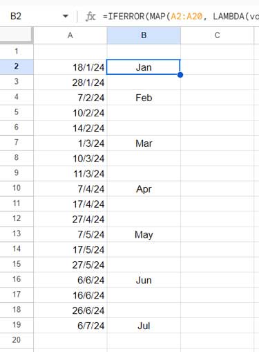

To display the full month names, replace “mmm” with “mmmm”.

For displaying the month & year at month change rows, you can utilize formats like “mmm-yy”, “mmm-yyyy”, “mmmm-yyyy”, etc.

For Excel, the formula varies slightly from the Google Sheets version. We will discuss this difference later in the tutorial.

Excel Formula:

=IFERROR(MAP(A2:A20, LAMBDA(val, IF(EOMONTH(DATEVALUE(TEXT(val, "YYYY-MM-DD")), 0)<>IFERROR(EOMONTH(OFFSET(val, -1, 0), 0), ""), TEXT(EOMONTH(val, 0), "mmm"), ""))),"")

Features:

• The formula doesn’t require sequential dates. For sequential dates, you can use simple logical tests to find the 1st day of each month and identify month starts.
• The formula returns an empty value if it encounters a blank cell or text in the range.
• The formula doesn’t require a sorted date range.
• Being a dynamic array formula, you can easily expand the range to return month names at month start dates.
• The output is highly customizable, allowing you to display month names, month and year, or month start dates.

These are the formula features that display month names at the start of each month in both Excel and Google Sheets.

Differences in Month Start Formulas: Excel vs Google Sheets

To identify empty cells and text in the range, I used the DATEVALUE function.

In Excel, DATEVALUE supports only date strings, so I used DATEVALUE(TEXT(val, "YYYY-MM-DD")) in Excel, whereas DATEVALUE(val) suffices in Google Sheets.

That’s the only difference in the formulas.

There is one more place where the formula could fail, which is with IFERROR.

In Google Sheets, you can use the IFERROR wrapper like IFERROR(…), but in Excel, you must specify the value to return when the formula encounters an error, like IFERROR(…, ""). I managed this by following the latter syntax in Excel and Google Sheets.

Month Names in a Row at Month Start Columns

This scenario is most useful when displaying month names at each month change.

In a Gantt chart timescale, you might have sequential daily or weekly dates across a row.

You might know how to display month names in each cell corresponding to the dates across a row, but not specifically in the columns where the month changes occur.

You don’t need to worry about the formula; you can use our earlier formulas with just one adjustment.

In the previous Excel and Google Sheets formulas, we used a row offset because we wanted the month names to display at each change of the month row.

Here, you should apply a column offset because we want the month names in the columns where the month changes occur.

The date range for the example is B3:S3. Here is the formula for Google Sheets:

=IFERROR(MAP(B3:S3, LAMBDA(val, IF(EOMONTH(DATEVALUE(val), 0)<>IFERROR(EOMONTH(OFFSET(val, 0, -1), 0), ""), TEXT(EOMONTH(val, 0), "mmm"), ""))),"")

And this one for Excel:

=IFERROR(MAP(B3:S3, LAMBDA(val, IF(EOMONTH(DATEVALUE(TEXT(val, "YYYY-MM-DD")), 0)<>IFERROR(EOMONTH(OFFSET(val, 0, -1), 0), ""), TEXT(EOMONTH(val, 0), "mmm"), ""))),"")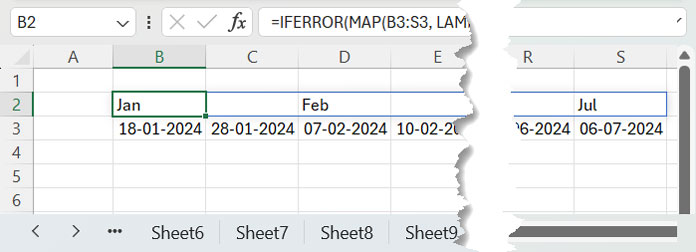

Formula Breakdown

Above, I’ve provided four formulas for dynamically displaying month names at month start, two for Google Sheets and two for Excel.

Since all the formulas follow the same logic, let me explain one of them. I’ll choose the last Excel formula, which you can see just above the screenshot.

The formula utilizes the MAP function to iterate a custom function across each row in the date range and return the month names in the columns where the month changes occur.

The formula operates as follows:

If the end-of-month date in cell B3 is not equal to the end-of-month date in cell A3, return the month text of the date in cell B3; otherwise, return an empty cell.

Formula:

=IF(EOMONTH(DATEVALUE(TEXT(B3,"YYYY-MM-DD")),0)<>IFERROR(EOMONTH(OFFSET(B3,0,-1),0),""),TEXT(EOMONTH(B3,0),"mmm"),"")

Where:

• EOMONTH(DATEVALUE(TEXT(B3,"YYYY-MM-DD")),0) returns the end-of-month date in cell B3.
• IFERROR(EOMONTH(OFFSET(B3,0,-1),0),"") returns the end-of-month date in cell A3.
• TEXT(EOMONTH(B3,0),"mmm") converts the date in cell B3 to the month’s abbreviated text.

To convert it to a custom function, we used the LAMBDA function, naming cell B3 as ‘val’ and using ‘val’ in the formula parts.

Here’s that custom function:

LAMBDA(val, IF(EOMONTH(DATEVALUE(TEXT(val, "YYYY-MM-DD")), 0)<>IFERROR(EOMONTH(OFFSET(val, 0, -1), 0), ""), TEXT(EOMONTH(val, 0), "mmm"), ""))

We have specified the array B3:S3 within MAP.

Syntax:

=MAP(array1,[array2],…,lambda)

The MAP function maps each value in this array to a new value by applying the LAMBDA function.

Resources

Here are a few resources that help you understand how the lambda helper functions and dynamic arrays differ in Excel and Google Sheets.

• Array Formula: How It Differs in Google Sheets and Excel
• BYCOL Differences: Sheets vs. Excel
• Google Sheets Vs Excel: BYROW – The Key Difference