The MAP function in Excel applies a custom LAMBDA function to each value in the given arrays, transforming each value into a new one.
Use the MAP function when you need to evaluate each value individually in a formula that doesn’t naturally spill in your Excel worksheet.
For example, you don’t need to use the MAP function to test whether each value in A1:A10 is greater than 49 and return “Passed” if it evaluates to TRUE and “Failed” otherwise. The following formula will accomplish that without MAP:
=IF(A1:A10>49, "passed", "failed")However, you might need to use MAP to convert the dates in A1:A10 to the end-of-the-month dates, as the following formula won’t work:
=EOMONTH(A1:A10, 0)This makes MAP one of the important functions for advanced data manipulations in Excel.
To summarize a dataset by week, month, year, quarter, etc., using a dynamic array formula instead of a pivot table or Power Query, you must rely on the MAP function.
Syntax and Arguments
MAP Function Syntax in Excel:
=MAP(array1,[array2],…,lambda)Arguments:
array1: The array to be mapped.array2: [Optional] Additional arrays to be mapped.lambda: A user-defined lambda function as per the syntaxLAMBDA(parameter1, [parameter2], …, calculation).
LAMBDA Function Details:
parameter1,parameter2,…: These are placeholders for the values that will be passed into the LAMBDA function. You can have one or more parameters depending on the number of arrays specified in the MAP function.calculation: This is the expression or calculation that uses the parameters.
Example 1: Using MAP with a One-Dimensional Array in Excel
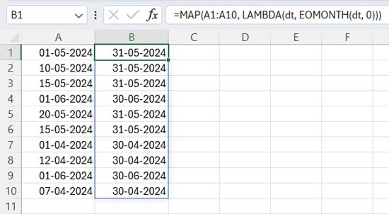
There are dates in A1:A10. The following MAP formula in cell B1 will return the end-of-the-month dates in B1:B10.
=MAP(A1:A10, LAMBDA(dt, EOMONTH(dt, 0)))The output of the above Excel formula will be date values. To format these dates, select B1:B10, and under the Home tab within the Number group, click the drop-down and select Short Date.
The purpose of this tutorial is to simplify the usage of the MAP function in Excel. So let me explain the above formula step by step before proceeding to the next example.
Formula Breakdown
The following formula returns the end-of-the-month date of the date in cell A1:
=EOMONTH(A1, 0)We can convert this formula to a custom LAMBDA function in Excel as follows:
LAMBDA(dt, EOMONTH(dt, 0))Where:
parameter1:dtcalculation:EOMONTH(dt, 0)
You’re free to use any meaningful name for parameter1 in the formula. There’s no need to stick to ‘dt’. If you use multiple words, either separate them with underscores or enter them without spaces, such as ‘DateToConvert’. This may help avoid using unsupported names.
Use the above custom function within the MAP for the array A1:A10, and that is our formula that returns the end-of-the-month dates.
Example 2: Using MAP with Two-Dimensional Arrays in Excel
Understanding how to use the MAP function with two-dimensional arrays is essential for mastering this function in Excel.
Here is a real-life scenario where we have the marks of two students in Model and Final exams for the subjects Maths, Physics, and Chemistry.
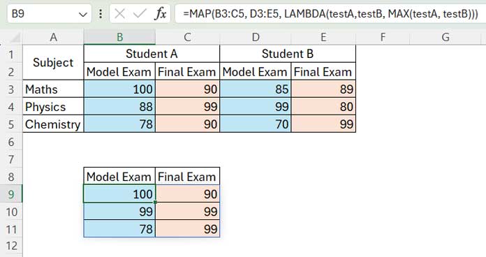
We will use the MAP function to find the best marks in these subjects separately in the Model and Final exams.
You can add as many students and subjects as you wish. For this example, we will stick with two students and three subjects.
Formula:
=MAP(B3:C5, D3:E5, LAMBDA(testA, testB, MAX(testA, testB)))Where:
array1: B3:C5 – The first array to be mapped.array2: D3:E5 – The second array to be mapped.lambda:LAMBDA(testA, testB, MAX(testA, testB))– The custom LAMBDA function.
You can understand this lambda function in a clever way. See what the following formulas return and the reasons. That will help you grasp the usage of the above MAP formula in Excel.
Formula Experiment 1:
=MAP(B3:C5, LAMBDA(testA, MAX(testA)))This formula will return the array as it is since it feeds one value at a time to MAX, like MAX(B3), MAX(C3), …
Formula Experiment 2:
=MAP(B3:B5, D3:D5, LAMBDA(testA,testB, MAX(testA, testB)))This will return the maximum of the pairs like MAX(B3, D3), MAX(B4, D4), and MAX(B5, D5) in the first, second, and third rows.
Now, for the real formula in the example:
=MAP(B3:C5, D3:E5, LAMBDA(testA, testB, MAX(testA, testB)))This will return the maximum of each pair, like MAX(B3, D3) and MAX(C3, E3) in two cells in row #1, then MAX(B4, D4) and MAX(C4, E4) in two cells in row #2, and finally MAX(B5, D5) and MAX(C5, E5) in two separate cells in row #3.
Resources
Here are some tutorials that use the MAP function in real-life Excel applications.
- Sum by Week Number in Excel (Dynamic Array Formula Included)
- Sum By Month in Excel: New and Efficient Techniques
- Sum By Quarter in Excel: New and Efficient Techniques
- Sum Values by Month and Category in Excel


