When you delete rows, it’s essential to double-check that you’re not losing any data. Let’s see how to delete empty rows in Google Sheets properly without affecting your important information.
When you clean up your data by removing duplicates or outdated transactions, you often create several blank rows. It’s a good idea to remove these blank rows to keep your data tidy and organized.
There are a few other advantages to deleting empty rows in Google Sheets, including:
- Free up space. Removing empty rows can free up space and improve your sheet’s performance. It also makes your sheet easier to navigate.
- Improve the performance of array formulas. Deleting empty rows can boost the efficiency of array formulas and LAMBDA functions by reducing the amount of data they need to process.
- Neat printout. If you plan to print your sheet, deleting empty rows will make your printout look cleaner and more professional.
- Simplify charts and pivot tables. You can avoid the hassle of filtering out empty rows when creating charts or pivot tables.
How to Delete Empty Rows in Google Sheets
To delete empty rows, we’ll follow this simple approach:
- Filter the data range to display only empty rows.
- Select and delete all empty rows in the sheet.
- Remove the filter.
This way, the sheet will contain only data rows. Here are the step-by-step instructions:
1. Set Up the Sample Data
For this test, I’ll use the following sample data in the range A1:G9.
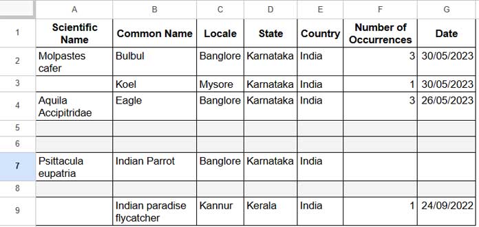
There are three blank rows in this range.
2. Filter Out Non-Empty Rows
To delete empty rows, first we need to filter out all non-empty rows.
What is a non-empty row?
A row is considered non-empty if there is a value in at least one of its columns. If all cells in a row are blank, it’s an empty row.
To filter out the non-blank rows in the range:
- Select A1:G9.
- Click Data > Create a filter.
- Click the filter drop-down in the top-left cell, which is A1.
- Select Filter by condition > Custom formula is.
- Enter:
=NOT(COUNTIF(A2:G2, "<>")) - Click OK.

Now, only empty rows will be displayed.
3. Delete Empty Rows
After filtering to show only the blank rows, delete them as follows:
- Click the row number of the first blank row (e.g., row #5).
- Press and hold the Shift key.
- Click the row number of the last blank row you want to delete (e.g., row #8).
(If you have more blank rows further down, scroll and select them as needed.) - Right-click the selected rows and choose Delete selected rows.
4. Remove the Filter
- Click Data > Remove filter.
Now you’ll have a clean dataset without any empty rows!
By following this method, you can easily learn how to delete empty rows in Google Sheets without losing any valuable data.


